

Learn through the super-clean Baeldung Pro experience:
>> Membership and Baeldung Pro.
No ads, dark-mode and 6 months free of IntelliJ Idea Ultimate to start with.
Learn through the super-clean Baeldung Pro experience:
>> Membership and Baeldung Pro.
No ads, dark-mode and 6 months free of IntelliJ Idea Ultimate to start with.
In this tutorial, we’ll talk about how the blur operation works in images. First, we’ll present kernel convolution, which is the basic operation behind any blur operation. Then, we’ll define two types of blur, the mean and the Gaussian blur, and provide some illustrative examples.
The most common operation in the field of computer vision and image processing is kernel convolution.
Formally, convolution is a mathematical operation where two functions are combined to generate a third function that expresses how the shape of one is influenced by the other. Its applications are numerous in various fields like statistics, signal processing, physics, acoustics, and so on. In our case, we focus on kernel convolution, which is the convolution between an input image and a small grid of numbers defined as the kernel.
So, in kernel convolution, we pass the kernel over the input image, transforming each time a pixel of the image based on a specific operation between the kernel and the corresponding pixels of the image. More specifically, for every pixel in the input image, we center the kernel over it and perform an elementwise multiplication between the pixels of the filter and the corresponding pixels of the image. Then, we sum up these values into a single value. Finally, we normalize the results by dividing them by the total value of the kernel to ensure that the intensity of each pixel is not influenced.
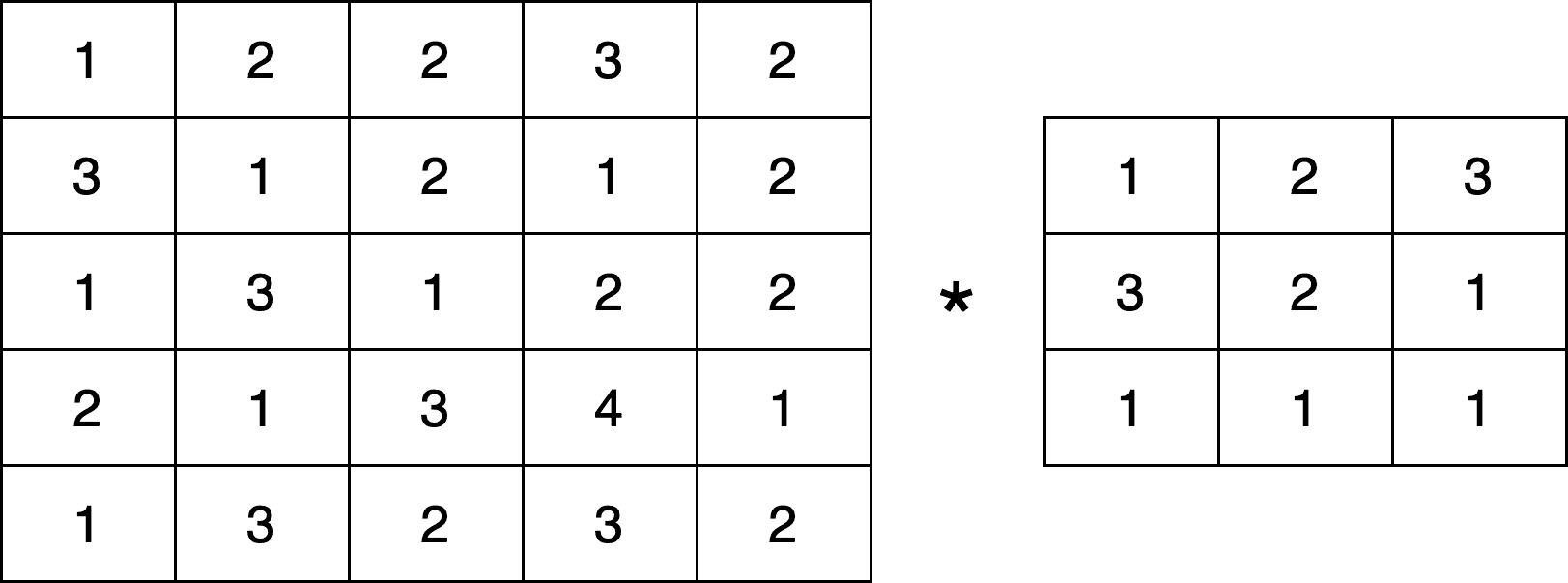
Let’s see an example to better illustrate the procedure. We assume that we have an input image  of size
  and a kernel
  of size
  , and we want to compute the convolution
  . Below, we can see some example inputs:
We’ll present one step of the procedure since the rest of the procedure is repeated iteratively for every pixel. Let’s choose the pixel  that is in the second row and column of the image and is equal to 1 (pink in the image below):
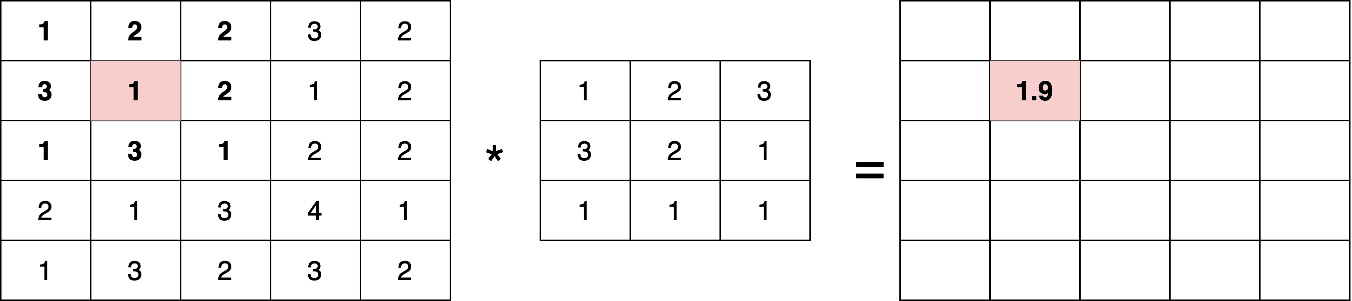
As previously presented, we first compute the multiplications between the pixels around the region of and the kernel . Then we sum the outputs:


Finally, we divide the output by the sum of the values of the kernel:

Intuitively, in kernel convolution, we compute a weighted average between regions of the input image and the kernel. In this article, we will see two types of kernels that aim to blur the input image.
If we set all the values of the kernel to 1, we end up with a mean blur operation to the input image, which is a very simple form of a blur. To better illustrate the mean blur, let’s compute the mean blur convolution of the previous image with a kernel of size 3. We should not forget that we talk about images, and the output pixels should always be integer values. So, we round the output of the final division to the closest integer:
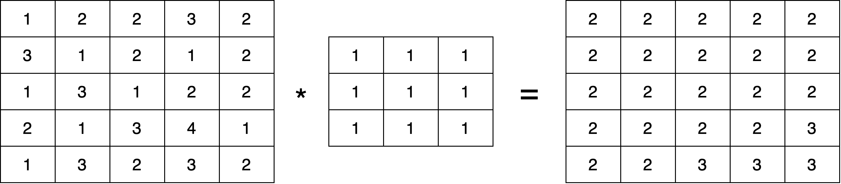
We can see that the mean blur makes the example image smoother. Below, we can see some examples of mean blurs in a real image with different values of the kernel size :
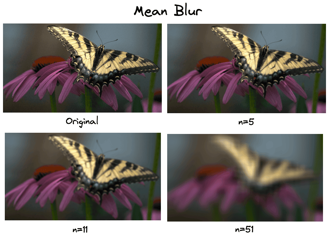
We can see that an important problem of mean blur is the fact that it doesn’t take into account the edges of the image. So, after blurring an image, its edges disappear.
To deal with the above problem, we can use the Gaussian blur that uses a slightly more complicated kernel, the Gaussian kernel.
Gaussian blur is the most common type of blur since it is edge-preserving. As the name suggests, it behaves like the Gaussian distribution giving more weight to the central pixels. An example Gaussian kernel of size has the below format:
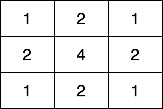
So, we can see that the major difference between Gaussian blur with the mean blur is the fact that it prioritizes the pixels in the middle of the region. The further we go from the central pixels, the less weight we have in the respective pixel of the input image::
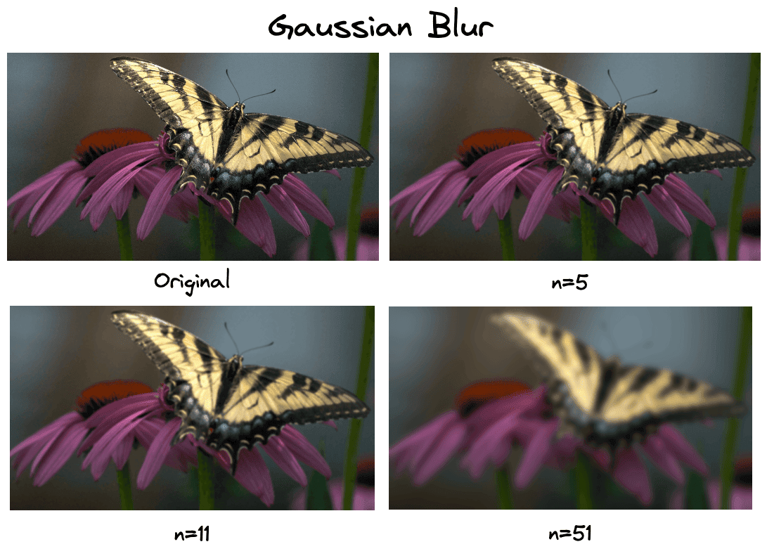
We observe that more edges are preserved in contrast with the mean blur operation.
In this article, we talked about how the blur operation works in images. First, we introduced the term kernel convolution, which lies at the heart of every blur operation. Then, we presented the mean and the Gaussian blur, along with some examples.