

Yes, we're now running our only Summer Sale. All Courses are 30% off until 20th July, 2026:
Learn through the super-clean Baeldung Pro experience:
>> Membership and Baeldung Pro.
No ads, dark-mode and 6 months free of IntelliJ Idea Ultimate to start with.
1. Introduction
Statistics is a powerful tool that enables us to make sense of data and draw meaningful conclusions from it.
In this tutorial, we’ll introduce the Student’s  -distribution, a generalization of the normal distribution named after the pseudonym “Student” used by William Gosset.
The Student’s -distribution steps in cases when dealing with small sample sizes or when the population variance is unknown. It provides a more accurate representation of the variability in sample means and enables making reliable inferences, even in situations where the standard normal distribution fails.
2. Definitions
2.1. Defining the Student’s t-Distribution
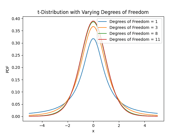
The t-distribution is a probability distribution that describes the variability of sample means when drawing random samples from a population. It forms a bell-shaped curve, similar to the normal distribution, but with heavier tails, which allows the -distribution to handle the increased uncertainty associated with small sample sizes.
The graph demonstrates that there is less space around the mean and more space in the -distribution’s tails. As a result, under the -distribution, more extreme values or outliers are more likely to happen:
2.2. Degrees of Freedom and Shape
The dependency of the -distribution on a variable known as degrees of freedom is one of its distinguishing characteristics. Degrees of freedom are a key factor in determining the distribution and indicate the number of samples of the sample. The -distribution approaches the form of the conventional normal distribution as the degrees of freedom grows.
The -distribution has broader tails than the normal distribution when the degrees of freedom are minimal, which increases the chance of extreme results. When working with sparse data, this feature is especially helpful since it more accurately depicts the intrinsic variability in sample means. Moreover, critical values are provided for various degrees of freedom and confidence levels in the -distribution table.
2.3. Deriving the t-Statistic
The foundation of the -distribution is the t-statistic, which measures the difference between the sample mean  and a hypothesized population mean
  in terms of the standard error of the sample mean.
3. Calculating and Using t-Scores
Let’s delve into the practical mechanics of calculating t-scores.
3.1. Step-by-Step Calculation of t-Scores
Calculating a -score involves quantifying the difference between a sample mean and a hypothesized population mean in terms of standard error. The formula for calculating the t-score is:
(1) 
where, t, , , s, n denote the t-score, the sample mean, the hypothesized population mean under the null hypothesis, the sample standard deviation, and the sample size, respectively.
3.2. Interpreting t-Scores
It’s critical to analyze the -score’s significance after we’ve calculated it.
Greater divergence from the anticipated mean is indicated by a bigger absolute t-score, and lesser deviation is shown by a lower -score. Also, we compare the -score to crucial values from the -distribution table depending on the degrees of freedom and the specified confidence level to ascertain whether the observed difference is statistically significant. Moreover, we may reject the null hypothesis if the estimated -score is greater than the critical value threshold since it indicates that the observed difference is probably not the result of chance.
3.3. Hypothesis Testing and Confidence Intervals
-scores are utilized in hypothesis testing for evaluating sample statistics to population parameters that are hypothesized. The estimated -score must be outside of the acceptance zone in order to successfully reject the null hypothesis. In contrast, if the -score is within the rejection range, there is no reason to accept the alternative over the null hypothesis.
-scores are used to calculate the margin of uncertainty surrounding the sample estimate when building confidence intervals. Higher uncertainty is shown in a broader confidence interval, whereas higher accuracy is reflected in a smaller interval.
4.
Let’s consider a practical example: a manufacturer wants to test whether a new production method improves the tensile strength of a certain material. A sample of 20 specimens is tested, yielding a sample mean tensile strength of 450 MPa, with a sample standard deviation of 25 MPa. The company believes the current tensile strength is 440 MPa. Using a significance level of 0.05 and a two-tailed test, we calculate the t-score:

With 19 degrees of freedom (20 – 1), we consult the -distribution table to find the critical value for a 0.025 significance level (0.05 divided by 2 for a two-tailed test), which is approximately 2.093. Since 2.52 exceeds 2.093, we reject the null hypothesis and conclude that the new production method likely results in a significantly higher tensile strength.
Moreover, consider an example where we are comparing the test scores of two groups of students using an independent t-test. Group A consists of 15 students and Group B consists of 18 students. The degrees of freedom for this test would be  .
.
5. Use Cases
The Student’s -distribution is more than just a mathematical curiosity; it’s a powerful tool with practical applications in a wide range of statistical analyses. The -distribution’s flexibility makes it a valuable tool in fields such as medicine, social sciences, engineering, and finance. Whether estimating treatment effects, analyzing survey data, or evaluating the performance of financial portfolios, the -distribution empowers analysts to draw reliable conclusions from limited information.
For example, researchers in medicine might use the -distribution to assess whether a new drug treatment yields a statistically significant improvement over an existing treatment, even when the sample size is limited.
Also, in marketing, analysts might use the -distribution to estimate the average response time of customers to an online advertisement, along with a confidence interval that quantifies the level of uncertainty around the estimate.
6. Conclusion
In this article, we discussed the Student’s -distribution as a useful tool, helping through the difficulties of uncertainty and variability in cases where data is frequently limited or sparse. It offers the ability to discover significant concepts and patterns, make wise choices, and increase knowledge in a variety of domains.