Converting a Uniform Distribution to a Normal Distribution

1. Overview

In this tutorial, we’ll study how to convert a uniform distribution to a normal distribution.

We’ll first do a quick recap on the difference between the two distributions.

Then, we’ll study an algorithm, the Box-Muller transform, to generate normally-distributed pseudorandom numbers through samples from the uniform distribution.

At the end of this tutorial, we’ll know how to build a pseudorandom generator that outputs normally-distributed values.

2. Uniformity and Normality

The first point in this discussion is to understand how a uniform and normal distribution differ. This lets us concurrently understand what we need to transform one into the other and vice-versa.

2.1. The Uniform Distribution

The uniform distribution also takes the name of the rectangular distribution, because of the peculiar shape of its probability density function:

Within any continuous interval $[a, b]$ , which may or not include the extremes, we can define a uniform distribution $U(a, b)$ . This is the distribution for which all possible arbitrarily small intervals $\epsilon \in [a, b]$ , with or without extremes, have the same probability $P(\epsilon) = \frac {1} {b-a}$ of occurrence. We can verify that this is a proper probability desity function by calculating the area under the curve:

$Pr[a \leq x \leq b] = \int_a^b \text{PDF}(x) dx = (b-a) \times \frac {1} {b-a} = 1$

2.2. The Normal Distribution

The normal distribution, instead, is a distribution characterized by this probability density function:

$\text{PDF}(x|\sigma, \mu) = \frac {1} {\sigma \sqrt{2\pi}} \times e^{-\frac{1}{2} (\frac{x-\mu}{\sigma})^2}$

In here, $\sigma$ and $\mu$ indicate, respectively, the standard deviation and the mean of the distribution. This is its corresponding chart, for $\sigma=1$ and $\mu=0$ :

We can see that the values contained in a normal distribution aren’t equally likely, as the corresponding values of the uniform distribution were. This is due to two reasons.

The first reason is that the uniformly-distributed values with non-zero probability are all contained in a finite interval, while those of the normal distributions aren’t. We noted that the values with a non-zero probability in the normal distribution occupy the whole domain $(-\infty, \infty)$ . This isn’t true for the uniform distribution, so we’ll need some kind of transformation to convert the finite interval $[a, b]$ to the other.

The second reason is that all values in discrete uniform distributions have the same probability of being drawn. For discrete normal distributions, instead, any two values $x_1 \neq x_2$ have corresponding probabilities $P(x_1) \neq P(x_2)$ different from one another. Of course, with the exception of the case in which $\frac {x_1 + x_2} {2} = \mu$ .

3. Box-Muller Transform

3.1. The Definition of the Algorithm

We can therefore identify an algorithm that maps the values drawn from a uniform distribution into those of a normal distribution. The algorithm that we describe here is the Box-Muller transform. This algorithm is the simplest one to implement in practice, and it performs well for the pseudorandom generation of normally-distributed numbers.

The algorithm is very simple. We first start with two random samples of equal length, $u_1$ and $u_2$ , drawn from the uniform distribution $U(0,1)$ . Then, we generate from them two normally-distributed random variables $z_1$ and $z_2$ . Their values are:

$z_1 = \sqrt{-2 \ln (u_1)} \cos (2 \pi u_2)$
$z_2 = \sqrt{-2 \ln (u_1)} \sin (2 \pi u_2)$

3.2. Empirical Testing

We can empirically test whether the procedure grants us a normally distributed random variable or not. This is done, concretely, by plotting the histogram of a bivariate distribution $u_1, u_2$ drawn from the uniform distribution. Then, we can compare it with the histogram of the corresponding transformed distributions:

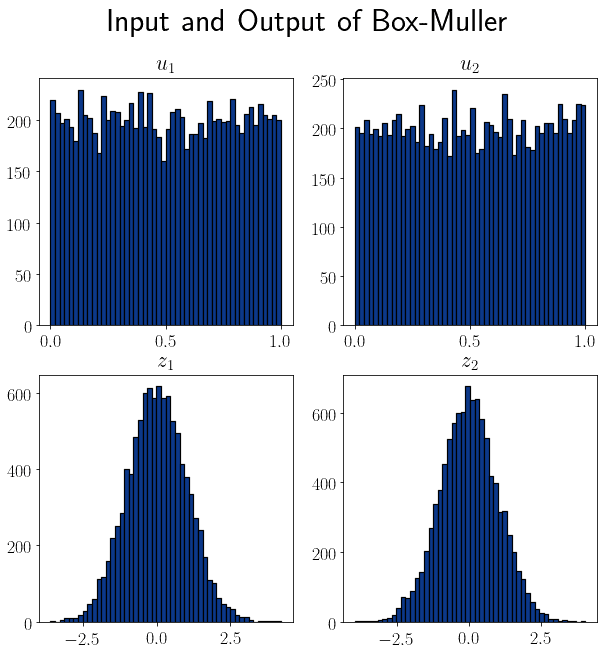
We made the charts above with two random samples $u_1, u_2$ of size 10,000. We can see that the corresponding distributions $z_1, z_2$ have the typical bell shape of a Gaussian distribution.

3.3. Deriving the Expression

We can understand how to derive the two expressions above if we imagine positioning the variables $u_1, u_2$ in the Cartesian plane. There, each of them corresponds to one of the two coordinates of a point:

Then, we can express the point in polar coordinates, identifying an angle $\theta$ and a distance of $r$ from the origin. This is because a bivariate normal distribution $(X, Y)$ has a norm $r$ that corresponds to $\sqrt{-2 \ln u_1}$ . Instead, the angle $\theta$ in the polar coordinates corresponds to $2 \pi u_2$ .

Finally, this lets us map the two variables $u_1, u_2$ in the original cartesian system to the normally-distributed variables $z_1, z_2$ , as:

$z_1 = r \cos(\theta)$

$z_2 = r \sin(\theta)$

Lastly, we can easily notice how these expression are equivalent to the ones we gave above.

3.4. The Limitations of Box-Muller

This algorithm performs well if we use it to generate a relatively short sequence of normally-distributed values. For a sufficiently short sequence, in fact, we expect most of its numbers to be contained within three standard deviations of the distribution’s mean. If, however, the sequence is large, we expect $\boldsymbol{\approx} \textbf{0.2\%}$ of the values to be located outside of that interval.

In computers with finite accuracy for the representation of decimal digits, there’s a limit to how close to zero can we draw a number from the uniform distribution. This changes depending on whether we use double or floating-point precision, but still implies a non-zero resolution to our capacity to draw from a continuous uniform distribution.

As a consequence, we can’t represent all possible values from the normal distribution by using the Box-Muller algorithm, but only those in sufficient proximity of the mean. A good rule of thumb is to state that the tail of the distribution truncates at $\approx 6.5$ standard deviations if we use 32-bits precision. If we use 64-bit precision instead, we can expect the generated values to be located within $\approx 9.5$ standard deviations.

3.5. Alternatives to Box-Muller

Alternatively, we can use other, more complex algorithms if we need to obviate the limitations of Box-Muller.

The first is the Ziggurat Algorithm, which uses the rejection sampling principle and generates normally-distributed values on the basis of a random seed and a lookup table.

The second is the Ratio-of-Uniforms, which demands the storage in memory of several double-precision values, but is otherwise computationally fast and simple.

The third is to calculate the inverse function to the cumulative distribution function for a normal distribution. This corresponds to calculating the quantile function of a normal distribution which, for standard normal distributions, coincides with the probit function.

4. Conclusion

In this tutorial, we studied how to generate a pseudorandom variable that’s distributed normally.

We did so by sampling from a bivariate uniform distribution and then applying the Box-Muller transform on them.

Full Archive

About Baeldung

Core Concepts

Operating Systems

Artificial Intelligence

Graph Theory

Latex