

Yes, we're now running our only Summer Sale. All Courses are 30% off until 20th July, 2026:
Learn through the super-clean Baeldung Pro experience:
>> Membership and Baeldung Pro.
No ads, dark-mode and 6 months free of IntelliJ Idea Ultimate to start with.
1. Overview
In this tutorial, we’ll study the idea of randomness and its applications to computer science.
We’ll first start by discussing the ontological and epistemological bases of randomness. Then, we’ll study the problems of random generation and random sampling.
At the end of this tutorial, we’ll be familiar with the reason why randomness is such an important concept in both computer science, statistics, and cryptography.
2. The Theoretical Bases of Randomness
2.1. An Introduction to the Theory of Randomness
Before we approach the practical applications of randomness in technology, it’s best to introduce its theoretical foundation. The concept of randomness, in its abstract form, is ill-defined, which means that there’s disagreement as to what pure randomness means. There’s however a general agreement on the idea of random phenomena and random sampling, so we can study them instead.
The concept of randomness is the subject of a joint study by philosophy, chaos theory, probability theory, and, in more recent years, computer science, artificial intelligence, and quantum computing. Its importance lies in the fact that many real-world technologies, such as cryptography and artificial swarm intelligence, require it as part of their theoretical foundations.
Randomness also has a deeper implication though. This is because it’s related to the idea that the result of events is aprioristically unpredictable. In science, the postulation of randomness prevents the deterministic reduction of nature to a predictable set of rules, as we’ll see shortly.
2.2. Not Only a Theory
But also, randomness plays an important role in the methodology, not just theory, of scientific research. This is because the validation of scientific hypotheses requires empirical testing. This, in turn, requires a method for solving the sampling bias of collected observations against a larger population; more on that later.
It’s however debated whether randomness exists in the real world, or whether it’s an artifact of the limited knowledge that humans possess. The first approach, the one that considers randomness as a property of nature, postulates the so-called “ontological randomness”. The second, the one that attributes it to the knowledge of the observer, assume instead “epistemological randomness”. We’re going to study both approaches in this first section of the article.
Once we understand the ontological and epistemological foundation for randomness, we’d then be able to comprehend its usage in practice, in the development of technologies based upon it.
2.3. A Non-Deterministic Universe
One of the oldest ideas about the world is that the universe, the kosmos, possesses an intrinsic order and perfection. This perfection corresponds to an arithmetical precision in the movement of stars, planets, and the life of humans that inhabit Earth. The idea takes the name of “determinism”, from the word terminus, definition or limit.
Determinism proved to be a fruitful approach to science, up until the first half of the 20th century. In physics, determinism allowed Newton to build his cosmological model, even though it was later falsified. In Newtonian mechanics, the universe acts as a clockwork mechanism in which all of its components behave in a determined and predictable manner:
Full and accurate predictions of the future of the universe are possible under this theory. The knowledge of the state of the universe in any given moment, and that of the rules that regulate its behavior, would, therefore, give complete knowledge of both the future and the past. We can thus say that Newtonian mechanics doesn’t allow for randomness.
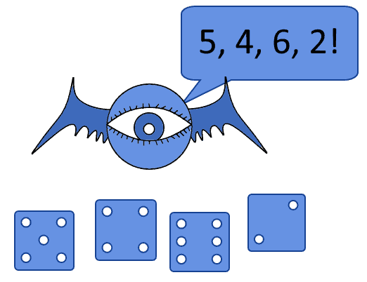
In a Newtonian universe, a being that possesses an accurate knowledge of the state and rules of the universe, such as Laplace’s demon, would, for all purposes, be omniscient. For that being, the result of any throw of dice would be known in advance, and hence there wouldn’t be any uncertainty about the future:
2.4. Chaos Theory and Randomness
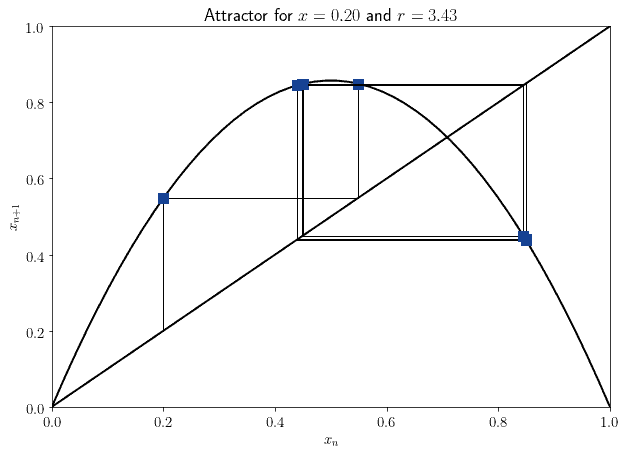
Absolute determinism was however falsified by chaos theory, which suggests that the evolutionary trajectories of the same system may vary wildly under analogous, but not identical, original states. Chaos theory suggests that a slight modification of the initial conditions of a system might result in completely different outcomes of its evolution. This is a concept known as sensitive dependence on initial conditions.
The most famous example of this concept is the logistic map  . The system is parameterized by
  , but is otherwise fully deterministic. Its behavior, however, changes dramatically according to its initial configuration; in this case, to the value of the parameter . This is the map of the so-called bifurcation diagram of the logistic map:
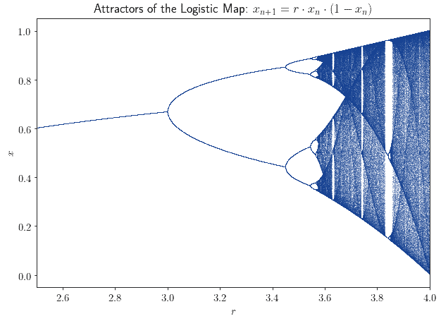
The behavior of the system might appear random for an observer. However, a simple deterministic rule exists from which its strange behavior descends. If therefore we knew the exact initial configuration of the system, we could then predict its future evolution with full precision:
From this consideration develops the idea that the behavior of a system might appear random, or not, according to the knowledge we have about that system. For an ignorant observer, a system might behave randomly. For a knowledgeable observer, the same system might behave deterministically. The idea of randomness as a property of an observer, or rather, of the knowledge he holds, starts to enter the scientific discussion.
2.5. Quantum Randomness
Another development of the idea of randomness derives from quantum mechanics, and in particular, from the famous double-slit experiment. This experiment showed that the act of measuring the state of a system, no matter which state or which system, modifies it. This, in turn, would invalidate predictions that might otherwise be sound.
Since the universe is, perhaps, a quantum system, this means that to determine the accuracy of any of our predictions, we need to conduct quantum measurements on the universe. This, in turn, would alter the state of the universe, subsequently invalidating them.
The question then becomes, how exactly a specific result for measurement is chosen. The Copenhagen interpretation suggests that, upon performing a measurement, one of the possible results is chosen randomly, and all other possible results are discarded. Here randomness enters into play physically, as a consequence of the interaction of an observer with a system.
2.6. Not One, but Many Worlds
Another idea is that randomness doesn’t exist at all, because the consequences of any event, whenever multiple of them are possible, all take place simultaneously. In the so-called Everettian interpretation, it’s proposed that random choice of the result of measurements doesn’t exist. Rather, all possible results of measurements are manifested simultaneously. However, only one is accessible to the observer.
In this context, the probability distribution of a random variable can be interpreted as a world-probability distribution. Imagistically, if we roll a die, the universe splits up and creates one copy of itself for any of the possible outcomes of our roll:
The observer would, however, perceive only the outcome of the roll related to the universe in which they exist.
While different interpretations disagree with the deeper meaning of the double-slit experiment, they all however agree in considering the role of the observer and observation as fundamental for the outcome of an event. This opens the doors to an epistemological, rather than an ontological, interpretation of randomness.
2.7. An Epistemological Justification
We can then follow this second route, and study randomness not as a property of the universe, but as a property of an event in relation to an observer. If the randomness of an event originates from the observer, then random events can’t be described as such without referencing one particular observer.
The randomness that two different observers would assign to the outcome of the same process might also differ. Let’s take the following example:
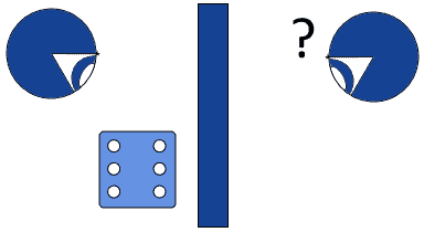
Behind a screen, the first observer rolls at a die and looks at its result. The second observer doesn’t see the result of the roll, initially. If the universe allows randomness, then the outcome of the roll is ultimately random for both observers. Once the first observer sees the result of the roll, though, is it random any longer?
We could say that, from the perspective of the second observer, the outcome is still random. If the second observer, however, learns the outcome, then we could argue that the roll’s randomness is gone:
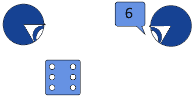
It seems, therefore, that a legitimate explanation of randomness would be linked to the knowledge held by an observer. As an observer acquires more knowledge about an event, its randomness might, then, decrease, or even disappear.
This example is an argument in favor of the so-called epistemological approach to randomness. In this context, randomness indicates only the uncertainty of a given observer about predictions or the result of some measurements but has no deeper, ontological meaning.
2.8. Why Does It Matter?
The ontological and epistemological foundation for randomness matters. This is because many important technologies, such as blockchain and encryption, need randomness to exist to function as intended. As we’ve seen above, it’s not so obvious that randomness has an ontological nature, and that it doesn’t refer instead to the state of an observer.
Unless the universe is intrinsically random, then we need to include a description of the observer when developing applications that exploit randomness. This is because in certain contexts, and in particular in the adversarial approach to encryption, different observers have different capacity to predict the future value of a random variable. As a consequence, they may disagree as to what variables they consider random, and why.
Suffice it to say, if randomness doesn’t exist, then we can’t build anything with it. And, as we saw earlier, it’s unclear that randomness is a property of the universe. It may, however, be a good way to measure uncertainty in predictions; and, in this sense, the theory of randomness finds its place among the theoretical bases for the development of technology.
3. Random Sequences and Random Generation
3.1. Randomness of Sequences
We’re now going to discuss the problem of generation and sampling of random variables. These are, in a practical sense, the two main branches in which we apply the theory of randomness.
In this section, we’re interested in understanding, when faced with a new sequence of numbers, whether that sequence is random or not. Let’s suppose that somebody tells us a single number:
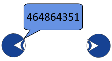
Is this number random? Its digits certainly look like they don’t have any relationship with one another, so we might suspect it is. Let’s ask some more numbers to the same person, just to check what happens next:
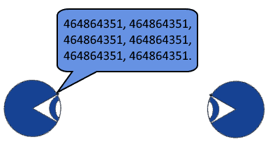
Whatever criterion our interlocutor follows to generate a number, it appears that the next number in the sequence is identical to all others. This means that any given number in the sequence has very limited, if any, information content.
Let’s now imagine that our interlocutor gives us another, new sequence:

This new sequence instinctually appears to be “more random” than the previous one. This is because, whatever procedure our counterpart follows to generate the sequence, we can’t easily guess it by looking only at the numbers themselves.
3.2. Random Generation
This consideration introduces us to the generation of random sequences. In ideal terms, we’d like a sequence of random numbers to have no algorithm, at all, that allows us to predict the next element in the sequence given the previous. If, however, we use an algorithm, any algorithm, to generate a sequence of numbers, the same algorithm, by definition, can compute any element in the sequence.
Unfortunately, we can’t procedurally generate numbers without an algorithm. As a consequence, the best thing we can do is to use some algorithm that makes reconstruction of the procedure we use particularly complex or costly. These algorithms take the name of “pseudorandom generators” because they don’t exploit true randomness, but rather an approximation of it.
3.3. Pseudorandom Generation: Middle Squares
The generation of pseudorandom numbers has been the concern of mathematicians such as Von Neumann. To him, we owe the discovery of the so-called middle square method, which allows the computation of an arbitrarily long sequence of pseudorandom numbers.
The method consists of the squaring of a given number, called “seed” of the sequence, and then in the extraction of the square’s middle digits. These middle digits then form the next number in the sequence, and on them we apply the same algorithm again and again. This table shows the computation of the first few elements in each sequence, for some seeds:

|

|

|

|

|

|

|
|---|---|---|---|---|---|---|
| 11 | 12 | 14 | 19 | 36 | 29 | 84 |
| 1234 | 5227 | 3215 | 3362 | 3030 | 1809 | 2724 |
| 1000 | 0000 | 0000 | 0000 | 0000 | 0000 | 0000 |
| 987654 | 460423 | 989338 | 789678 | 591343 | 686543 | 341290 |
This method is subject to a critical problem, though. This is apparent if we look at the third line, with seed “1000”, of the table above. If a zero appears as the middle digits in one of the numbers in the sequence, it’s going to stay there indefinitely. This means that the sequence, with a seed of 1000, converges to zero, which makes the algorithm useless with that particular seed.
Other pseudorandom generators possess even more critical issues. The dual elliptic curve pseudorandom generator, for example, has been involved in controversies regarding the actual predictability of the numbers it generates. After being proven vulnerable, it was eventually withdrawn from the market, due to a hidden trivial method for predicting its future output.
This means that the method we choose to generate random numbers matters and that we might end up with trivial sequences if we’re not careful. We can thus conclude this section with the words of Dr. Knuth, who said that a random number shouldn’t be generated with a random method, but that some theories should be used instead.
4. Random Sampling
4.1. Random Sampling and Statistics
Randomness also helps us study the characteristics of a population, on the basis of those of a smaller sample, while avoiding mistakes due to bias. If we randomly sample a large dataset, the statistics of the sample tend to those of the population as the sample size increases:
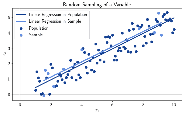
This is generally valid for all statistics and all populations. The selection of the sample must however be performed randomly, or this rule won’t be valid.
4.2. Non-Random Sampling
We can in fact see what happens when we don’t sample randomly. As a general rule, the non-random sampling leads to gross errors in the statistics computed on that sample.
Let’s demonstrate this with a small experiment, in which we conduct non-random sampling over the data points of the previous image. We might, for example, arbitrarily decide to take the 10 closest observations to the median value and compute a statistic on them:
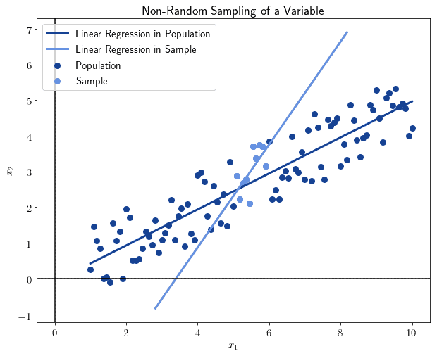
We can see that the result differs significantly from the previous. And this isn’t random: the non-random selection of the sample leads to a distortion of the results and a loss of representativeness over the general population.
4.3. Distribution of Random Variables
We can now discuss the shape of the distribution of random variables. Some shapes are particularly intuitive to understand. If, for example, we randomly sample  of size
  from the uniform distribution (0, 1), then is also uniformly distributed:
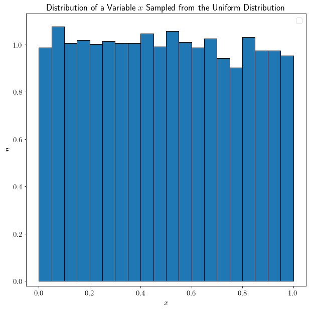
Short of stochastic variability, an approximately equal number of draws fall into any arbitrarily selected sub-intervals of the uniform distribution of equal size. We could also sample from the normal distribution instead; and again, the resulting variable would have a normal shape, just like the sampled distribution:
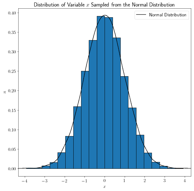
As a general rule, the variable , randomly sampled from a distribution  , has the same shape of .
4.4. Combinations of Random Variables
The rule that’s valid for a single variable doesn’t hold true, however, for multiple variables and their linear combinations. We can test this experimentally. Let’s assume that and  are random variables that we sampled from a uniform distribution. We can thus study their linear combination
  :
:
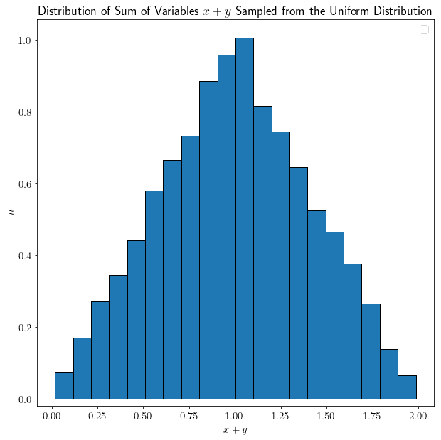
Surprisingly, their sum is no longer uniformly distributed, but rather it’s assuming a very peculiar shape. Let’s repeat the experiment, by adding a third variable  that we also sampled from a uniform distribution:
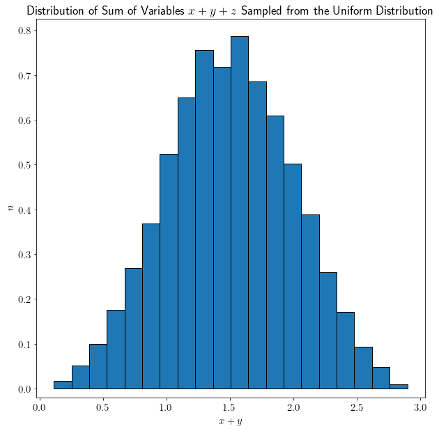
Now the shape becomes more prominent. Let’s finally repeat the experiment with 100 variables  sampled from the uniform distribution:
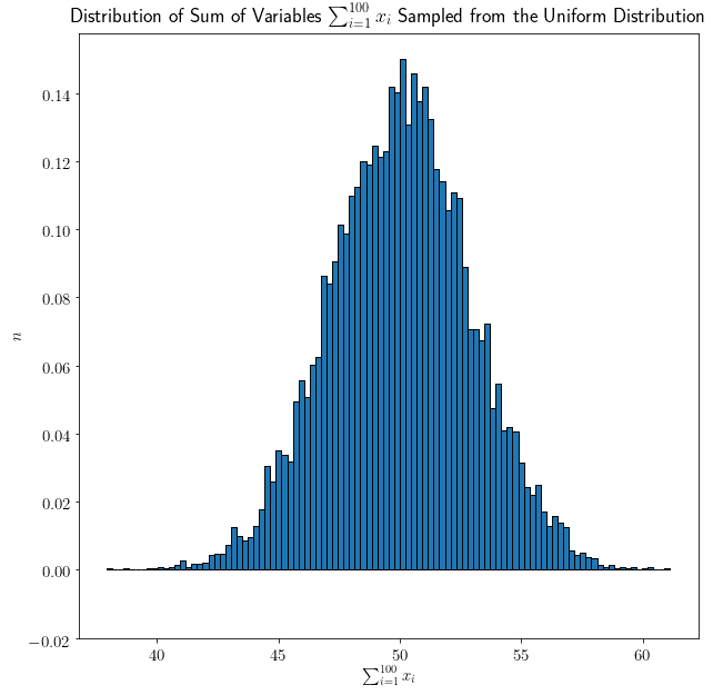
Now the shape appears clearer, and it looks exactly like a normal distribution.
4.5. The Central Limit Theorem
We can formalize in mathematical terms the observation we made above, which takes the name of the central limit theorem. The theorem states that, as the number of random variables that we consider increases, no matter the shape of the distribution that generated them, their sum tends towards a normal distribution.
We can express the theorem with formal notation. If  indicates the average for the variable
  , and if
  and
and  indicate, respectively, the mean and the standard deviation of the distribution from which all ‘s are drawn, then the distribution
  of the sum of all can be expressed as:

Where  is the normal distribution.
4.6. Application of the Central Limit Theorem
We can best understand the importance of this theorem with a practical example. Let’s sum the result of the roll of two dice,  and
and  . We might expect that, since the original two dice are uniformly distributed in the interval
 ![[1, 6]](/wp-content/ql-cache/quicklatex.com-d87268f303832e9d5e989bedfe47537c_l3.svg "Rendered by QuickLaTeX.com") , then the sum
, then the sum  will also be distributed uniformly in the interval
 ![[2, 12]](/wp-content/ql-cache/quicklatex.com-817ce3dca871096f914dc49889f98030_l3.svg "Rendered by QuickLaTeX.com") .
.
This is the distribution of the sum of two dice, though, which proves the hypothesis to be incorrect:
| + | 1 | 2 | 3 | 4 | 5 | 6 |
|---|---|---|---|---|---|---|
| 1 | 2 | 3 | 4 | 5 | 6 | 7 |
| 2 | 3 | 4 | 5 | 6 | 7 | 8 |
| 3 | 4 | 5 | 6 | 7 | 8 | 9 |
| 4 | 5 | 6 | 7 | 8 | 9 | 10 |
| 5 | 6 | 7 | 8 | 9 | 10 | 11 |
| 6 | 7 | 8 | 9 | 10 | 11 | 12 |
And this is the same content of the table above, in the form of a chart:
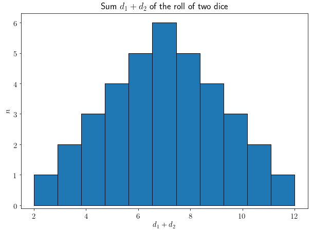
We can see that the normal shape of the distribution already starts to emerge when we sum just two dice. If we sum more than two dice, the central limit says, the Gaussian shape will only become more prominent.
5. Conclusions
In this article, we first studied the ontological and epistemological foundations of randomness.
Then, we studied how random generation and random sampling differ from one another in their practical applications for computer science.