Yes, we're now running our only Summer Sale. All Courses are 30% off until 20th July, 2026:
Importance of Statistics in Machine Learning
Last updated: February 28, 2025

Learn through the super-clean Baeldung Pro experience:
>> Membership and Baeldung Pro.
No ads, dark-mode and 6 months free of IntelliJ Idea Ultimate to start with.
1. Introduction
In this tutorial, we’ll understand the discipline of statistics and how it is a valuable tool in data science. We’ll begin by exploring general concepts and classifications of statistics and proceed to cover some of the popular statistical tools of interest in machine learning.
Statistics is developing and studying methods for collecting, analyzing, interpreting, and presenting data. More particularly, statistics is concerned with using data for decision-making in the context of uncertainty.
2. Basic Concepts in Statistics
Before we understand how statistics plays a vital role in machine learning, we must go through some of the fundamental concepts in statistics. These concepts form the basis of any statistical analysis, and we’ll often hear about them.
2.1. Population and Sample
The application of statistics starts with a statistical population, which represents a set of similar items or events that interest some question or experiment. For instance, “all people living in a country” or “every atom composing a crystal”:
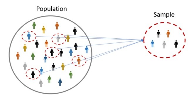
If a population is large, statisticians often choose a subset of the population, called a statistical sample. For instance, “a thousand residents of a country”. Of course, we must be careful to choose an unbiased sample that accurately models the population.
2.2. Probability Distribution
Probability distribution is an important concept in statistics as it helps us to describe the populations of real-life variables, like the age of every individual in a city. It’s a mathematical function that gives the probabilities of the occurrence of different possible outcomes for an experiment:
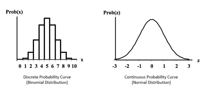 The variable in consideration can be discrete or continuous. Hence, the probability distribution can be described by a probability mass function or a probability density function. Some popular probability distributions include the Standard distribution and the Binomial distribution.
2.3. Central Limit Theorem
Central Limit Theorem (CLT) states that for independent and identically distributed random variables, the sampling distribution of the standardized mean tends towards the standard normal distribution even if the original variables themselves are not normally distributed:
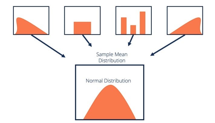
There have been several variations of CLT proposed over time. However, it remains a fundamental concept in the statistical analysis of data. This is because it helps estimate the population’s characteristics based on samples taken from it.
3. Methods of Statistical Analysis
We can use two main methods for statistical analysis of the sample data drawn from a population – descriptive statistics and inferential statistics. While descriptive statistics aims to summarize a sample, inferential statistics use that sample to learn about the population.
3.1. Descriptive Statistics
Descriptive statistics is the process of using and analyzing the summary statistic that quantitatively describes or summarizes features from a sample. Descriptive analytics provide simple summaries of the sample in the form of quantitative measures or visual graphs.
Some measures we often use to describe a data set include measures of central tendency, variability or dispersion, and actions of the shape of a probability distribution. Then several statistical graphic techniques further aid in visually describing the data set.
Descriptive statistics techniques are pretty helpful in performing empirical and analytical data analysis. In fact, exploratory data analysis (EDA) is an approach to analyzing data sets that package a collection of different summarization techniques.
3.2. Inferential Statistics
Inferential statistics is the process of using data analysis to infer the properties of a population. Here, we assume the observed data set is sampled from a larger population. Inferential statistics is based on probability theory, which deals with the analysis of random phenomena.
A statistical inference requires some assumptions. Thus, a statistical model is a set of beliefs concerning generating the observed data. Statistically, statisticians use many levels of modelling assumptions, for instance, fully parametric, non-parametric, and semi-parametric.
The conclusion of statistical inference is a statistical proposition. A statistical proposition can take many forms, like a point estimate, an interval estimate or a confidence level, a credible interval, rejection of a hypothesis, and clustering or classification of data points into groups.
4. Descriptive Statistical Tools
As we’ve seen earlier, descriptive statistics helps us to understand the data and hence it plays an important role in the machine learning process. We’ll go through some popular descriptive statistical tools that can help us ensure that the data meets the requirement for machine learning.
4.1. Measure of Central Tendency
In statistics, central tendency refers to the central value for a probability distribution. It may also denote the tendency of quantitative data to cluster around some central value. The three most widely used measures of central tendency are mean, median, and mode:
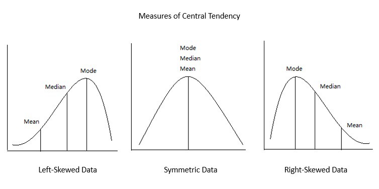
The sum of all measurements divided by the number of observations in a data set gives us its mean. The middle value that separates the higher half from the lower half of the data set is known as its median. Further, the most frequent value of the data set is known as its mode.
4.2. Statistical Dispersion
In statistics, dispersion refers to the extent to which a probability distribution is stretched or squeezed. A data set’s dispersion often indicates whether data has a solid or weak central tendency. The commonly used measures of dispersion are variance, standard deviation, and interquartile range:
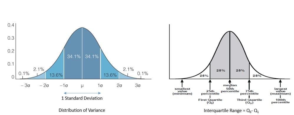
Variance is the squared deviation from the mean of a random variable. Further, variance is often defined as the square of the standard deviation. Interquartile range is the difference between the data’s 75th and the 25th percentile.
4.3. Shape of Probability Distribution
The shape of a probability distribution plays a vital role in determining an appropriate distribution to model a population’s statistical properties. This is often mentioned descriptively. For instance, the normal distribution is called the “bell curve”:
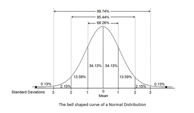
Then there are quantitative measures like skewness and kurtosis to describe the shape. Skewness is a measure of the asymmetry of the probability distribution of a random variable about its mean. Kurtosis is a measure of the “tailedness” of the probability distribution of a random variable.
5. Inferential Statistical Tools
Inferential statistics is about making inference about a population based on a sample taken from that population. The tools available in inferential statistics are of immense help in developing a machine learning model. These include important steps like feature selection and model comparison.
5.1. Hypothesis Testing
Statistical hypothesis testing decides whether the data sufficiently support a particular hypothesis. It allows us to make probabilistic statements about population parameters. A statistical hypothesis can be a statement like, “the office coffee dispenser is dispensing more than 100 ml”:
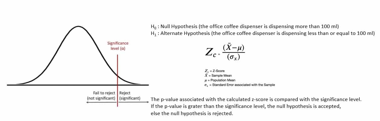
We begin by rephrasing our hypothesis as the null hypothesis ( ) and the alternate hypothesis (
 ). Then we collect sample data and conduct a statistical test like z-test. The statistical test provides us with the
  , which helps determine if the null hypothesis should be rejected.
5.2. Regression Analysis
Regression analysis is a set of statistical processes for estimating the relationships between a dependent variable and one or more independent variables. For instance, linear regression tries to find the line that most closely fits the data according to specific criteria like ordinary least squares:
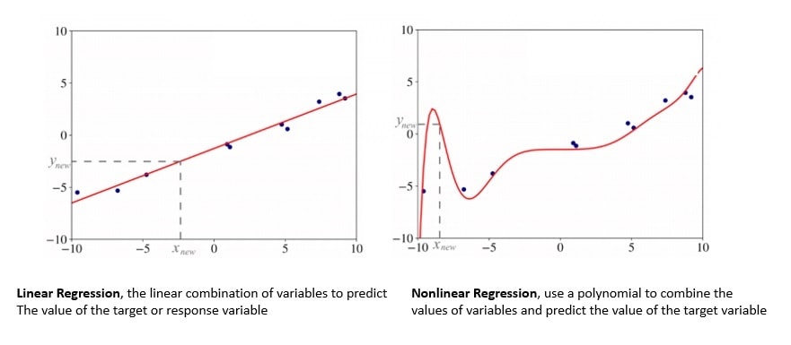
Then there is nonlinear regression in which the observational data are modelled by a function which is a nonlinear combination of model parameters and one or more independent variables. Regression analysis is widely used for prediction and forecasting and to infer causal relationships between variables.
5.3. Analysis of Variance (ANOVA)
Analysis of Variance (ANOVA) is a collection of statistical models used to analyze the differences among means. It’s based on the law of total variance, where the observed variance in a particular variable is partitioned into components attributable to different sources of variation:
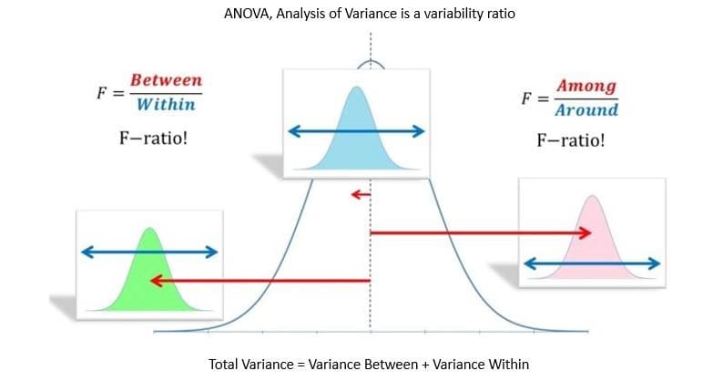
ANOVA provides a statistical test of whether two or more population means are equal. It’s beneficial to describe otherwise complex relations amongst variables. This method is often used in analyzing experimental data and has some advantages over correlation.
6. Paradigms in Inferential Statistics
Over time different paradigms of statistical inference have been established. Some statistical methods belong to a particular paradigm, while others find different interpretations under different paradigms. The most popular paradigms include the frequentist and the Bayesian paradigms.
6.1. Frequentist Inference
Frequentist inference is based on frequentist probability which treats probability in equivalent terms to frequency. It’s the study of probability, assuming that results occur with a given frequency over time or with repeated sampling.
Frequentism concludes sample data by means of emphasizing the frequency of finding in the data. Frequentist statistics provides well-established statistical inference methodologies, like statistical hypothesis testing and confidence intervals.
There are two complementary concepts in frequentist inference, the Fisherian reduction and the Neyman-Pearson operational criteria. Some key contributors to the formulation of frequentism were Ronald Fisher, Jerzy Neyman, and Egon Pearson.
6.2. Bayesian Inference
Bayesian inference is based on Bayes’ theorem, which is used to update the probability of a hypothesis as more evidence becomes available. Bayes’ theorem describes the probability of an event based on prior knowledge of conditions that might be related to the event:

Here,  stands for any hypothesis,
  is the prior probability of the hypothesis,
  is the new evidence,
  is the likelihood,
  is the marginal likelihood, and
  is the posterior probability. We are interested in calculating the posterior probability.
Hence, Bayesian inference uses the available posterior beliefs to make statistical propositions. The popular examples of Bayesian inference include credible intervals for interval estimation and Bayes factors for model comparisons.
7. Statistics in Machine Learning
Machine learning is a branch of Artificial Intelligence that focuses on using data and algorithms to imitate how humans learn, gradually improving its efficiency. It comprises of multiple stages, and statistical tools play a critical role in all the stages of machine learning:
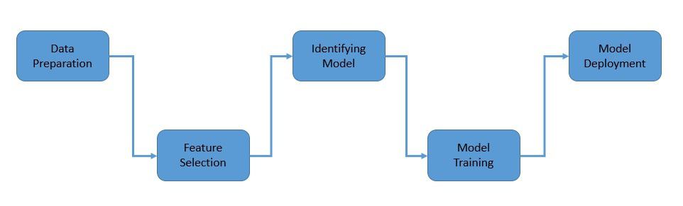
7.1. Data Preparation
As with many other aspects of computer science, machine learning is heavily influenced by the concept of Garbage In, Garbage Out (GIGO). It stipulates that flawed input data produces nonsense output, no matter the quality of algorithms used to process them in between.
For instance, a machine learning model trained on incomplete or biased data is poised to produce wrong or biased predictions. The data we collect to train our model must be relevant, representative, unbiased and anomalies-free.
The process begins by understanding the available data. Tools in descriptive statistics play an essential role in data exploration. Further, statistical devices like imputation and outlier detection help identify and remove data loss, errors and corruption.
7.2. Feature Selection
Feature in machine learning is an individual measurable property or characteristic of a phenomenon. For instance, the relative humidity of a location. Choosing informative, discriminating, and independent features is another crucial step for successfully applying machine learning algorithms.
Feature engineering is the process of transforming raw data into features that are suitable for machine learning models. It comprises of two processes, feature selection and feature extraction. It employs several statistical tools for selecting, extracting, and transforming the most relevant features.
The choice of tool depends on the nature of input and output data which can be either numerical or categorical. The available statistical tools include Pearson’s correlation coefficient, Spearman’s rank coefficient, ANOVA correlation coefficient, Kendall’s rank coefficient, and Chi-squared test.
7.3. Identifying Machine Learning Model
While statistical models are used for finding and explaining relationships between variables, machine learning models are built to provide accurate predictions without explicit programming. Although, statistical models are used extensively to arrive at an appropriate machine-learning model.
Machine learning models derive a lot of methodologies from statistics. For instance, the linear regression model leverages the statistical method of least squares. Even complex machine learning models like neural networks use optimization techniques like gradient descent based on statistical theory.
Several machine learning models are available, and it’s essential to choose the right one for the problem we want to solve. Again, statistics plays a vital role in model selection through tools like hypothesis testing and estimation statistics.
7.4. Model Training
The machine learning model needs to be fed with sufficient training data to learn from. This is an iterative process called model fitting. Here, the model gains efficiency in prediction by correlating the processed output against the sample output.
The objective is to identify the optimal set of model parameters and hyperparameters. While the model parameters are learned during training, the hyperparameters are adjusted to obtain a model with optimal performance.
Many statistical techniques are essential for validating and refining machine learning models. For instance, techniques like hypothesis testing, cross-validation, and bootstrapping help quantify the model’s performance and avoid problems like overfitting.
7.5. Model Deployment
A machine learning model needs to be evaluated in terms of its prediction quality. There are several statistical techniques which help us to quantify it. For instance, accuracy, precision & recall, F1 score, confusion matrix, and AUC-ROC curve, to name a few.
Once we’ve obtained an acceptable quality model, we need to use it for prediction on unseen data. However, like any other prediction, it can never be completely accurate. Hence, we’ve to quantify the accuracy using prediction and confidence intervals.
Finally, when the machine learning model is trained on the input data deployed for making predictions on new data, it needs to keep evolving. Statistics, like before, play an essential role in feeding the prediction accuracy back to update the model parameters accordingly.
8. Conclusion
In this tutorial, we went through the basic concepts of statistics. It included the broad categories of predictive and inferential statistics and some of the popular statistical tools within these categories available for us to use in machine learning.
Finally, we went through different machine-learning steps and understood how statistics plays a vital role in each step. It’s important to note that statistics forms the very foundation on which the machine learning process rests.