Outlier Detection and Handling

1. Introduction

Detecting and handling outlier values in the dataset is a critical issue in machine learning. As the supervised learning algorithms learn the patterns in the dataset, training with noisy datasets results in models with low prediction power.

Some algorithms, such as kNN, are more sensitive to outliers. On the other hand, tree-based methods, such as random forest, are more resilient to outlier values.

In this article, we’ll learn what outliers are. Then, we’ll discuss methods to detect them. Finally, we’ll consider how to handle them.

2. Outliers

In statistics, we call the data points significantly different from the rest of the dataset outliers. In other words, an outlier contains a value that is inconsistent or doesn’t comply with the general behavior.

Multiple reasons cause outliers to appear in a dataset. In this sense, a measurement error or an input error can lead to the existence of outlier values.

For example, we expect the age feature to contain only positive integers. An observation with an age value of “-1” or “abc” can’t exist. Hence, we conclude there’s a mistake.

On the other hand, when we have an age value of 112, it doesn’t have to be an erroneous entry. The datum is unusual, but it can still be valid. Removing that value would cause a loss in information.

In addition, outliers play an essential role in classification problems on imbalanced datasets. For instance, transactions in a fraud detection dataset are imbalanced. Moreover, the transactions deviating from the averages are more possibly the fraudulent ones. Hence, removing the outliers would again cause a loss of valuable information.

But conversely, the outliers introduce noise into a dataset and don’t prove helpful. We need to remove the observations that are not fitting into the dataset’s characteristics, especially when the number of observations is large. All in all, keeping them would lead to inadequately trained models.

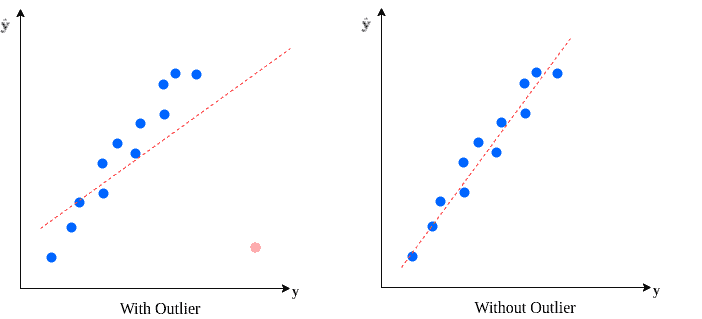
Let’s consider we fit a linear regression model on a dataset. Removing and not removing the outliers will have a considerable influence over the final model:

3. Outlier Detection

Detection of outliers isn’t a trivial problem. We’re trying to identify observations that don’t fit into the general characteristics of the dataset.

We can choose from a variety of approaches, depending on the dataset at hand. Let’s explore some of the well-known outlier detection techniques:

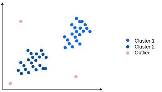
3.1. Data Visualization

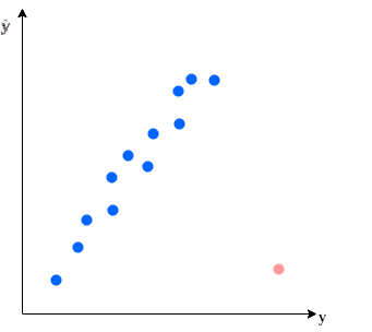
Data visualization is a simple and effective approach to detecting outliers. Especially when the dataset is low dimensional, we can easily generate a scatterplot showing outlier values:

However, as the dimensionality of the dataset increases, it’s harder to represent the dataset visually. Hence, it’s harder to detect outliers in a multi-dimensional dataset by visualization. So, we need to rely on other techniques, especially for high-dimensional datasets.

3.2. Quartile Analysis

Alternatively, we can mathematically define outlier candidates based on a feature’s statistical properties. Let’s first define some terms we’ll adopt.

A quartile divides the observations into four parts. is called the first quartile, and it represents the 25th percentile of the dataset. Similarly, denotes the third quartile and marks the 75th percentile of the data.

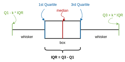
Progressing further, we define the interquartile range as:

In the quartile analysis method, we define the values falling outside the range to be outliers.

We can visualize the quantile analysis with the help of boxplots. The boxplot’s ends mark the quartiles. Additionally, the median is marked on the plot. The whiskers indicate the data range:

A commonly used value for the multiplier is 1.5. Hence, the values residing outside the 1.5 range are outliers:

3.3. Z-Score

Z-score measures the variance of an observation from the mean in terms of standard deviation, assuming a normal distribution.

To calculate z-score, we transform the data into a normally distributed bell curve, with mean and standard deviation . Then, we calculate the z-score of an observation :

Finally, we define a threshold range and mark the observations falling outside the range as outliers.

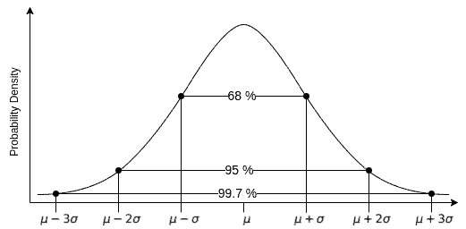
Let’s recall the empirical rule and coverage of standard deviation around the mean:

• covers 68.27%
• covers 95.45%
• covers 99.73%

Usually, we round the numbers and call the coverages to be 68 – 95 – 99.7:

Some common z-score threshold values are 2.5, 3.0, and 3.5. Based on the selected threshold value, we mark the observation with greater absolute z-scores as outliers:

3.4. DBSCAN Clustering

We can utilize a model to cluster the dataset. Then, the points that are too far away from the cluster centers would be outliers.

DBSCAN is a widely utilized clustering method for outlier detection. It is a non-parametric model. DBSCAN assumes that the clusters are dense. Hence, it investigates locally dense regions in a large dataset to detect clusters.

It classifies each point in the dataset as either a core, border, or noise point. With its output, we can easily identify the outliers marked as noise:

It’s a good practice to scale the dataset before applying a distance-based algorithm such as DBSCAN. Moreover, we need to choose a spatial metric depending on the dataset dimensionality.

3.5. Isolation Forest

Another method to detect outliers is using the isolation forest algorithm. The idea was first proposed for anomaly detection.

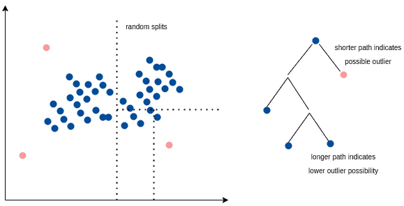
Isolation forest creates random partitions based on a feature. A tree structure visualizes how we form the splits. So, the number of edges from the root to a sample represents the number of splits required to isolate that particular observation.

The average path length of such trees serves as a decision function. We assign an anomaly score to all observations. The outliers have smaller path lengths, as they are easier to isolate. Conversely, non-outliers are harder to separate from the rest and have longer paths from the root.

Resultingly, when we form a forest of such random trees, they collectively produce a path length for a given observation. The collectively shorter averages are more likely to be outliers:

4. Handling Outliers

Detection and handling of outliers is a fundamental problem in data science and machine learning. Solving this problem isn’t straightforward, just like the missing values problem.

As we already mentioned, leaving the outliers as is reduces model performance. The model will learn the dataset patterns as well as the error and noise from the outlier values. Hence, we should remove them before the training phase.

There are several ways to handle an outlier value. Depending on the cause and density, we can select an appropriate method to address the outlier values. Still, correcting the value isn’t possible most of the time.

Suppose we believe that the observation results from a data entry error or a measurement error (“abc” in age field). Then, the best way of handling it is by removing the datapoint. Since we know that the data is invalid and incorrect, there’s no way to correct it.

We call replacing a data point with a substitution imputing. It’s common to predict the missing value based on other features or replace it with the feature mean to impute a value.

If the dataset is large enough, there’s a higher probability of seeing the extreme values (“114” in the age field). In this case, we can keep or trim the outlier value. For example, we can replace all values greater than 80 with 80 in the age example. This method is also called clipping or winsorizing.

Alternatively, we can use non-statistical methods to handle outliers. We can ask stakeholders and domain experts about the possible values of a feature. We can brainstorm with them to determine the reasons for the deviation of some observations from the rest of the dataset. Ideas shaped with domain knowledge lead to better solutions to the problem at hand.

5. Conclusion

In this tutorial, we’ve learned about outliers and why they are important. We’ve discussed some possible reasons for the existence of outliers in a dataset.

Then, we’ve learned about some of the most widely used methods to detect outliers. We covered data visualization, quartile analysis, z-score, DBSCAN clustering, and isolation forest methods.

Finally, we’ve discussed some methods for outlier handling and concluded.