Radial Basis Function | Baeldung on Computer Science

1. Introduction

In this tutorial, we’ll deep-dive into the ocean of radial basis function or RBF.

2. RBF

In a mathematical context, RBF is a real-valued function that we use to calculate the distance between a variable with respect to a reference point. In a network context, an RBF network is an artificial neural network in which we use the radial basis function as the activation function of neurons.

2.1. Definition

RBF is a mathematical function, say $\psi$ , that measures the distance $d$ between an input point (or a vector) $x$ with a given fixed point (or a vector) of interest (a center or reference point) $o$ .

$\psi(x) = d(||x-o||)$

Here, $d$ can be any distance function, such as Euclidean distance. Further, the function $d()$ depends on the specific application and desired set of properties. For the case of vectors, we call this function RBK (radial basis kernel).

We use RBF in mathematics, signal processing, computer vision, and machine learning. In these, we use radial functions to approximate those functions that either lack a closed form or are too complex to solve. In most cases, this approximation function is a generic neural network.

2.2. Types

RBF measures the similarity between a given data point and an agreed reference point. We can then use this similarity score to take specific actions, such as activating a dead neural network node. Over here, the similarity directly correlates with the distance between the data and reference points.

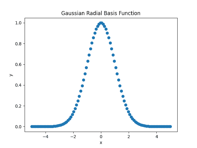
Depending upon the function definition, we can have different RBFs. One of the most commonly used RBFs is the Gaussian RBF. It is given by:

$\psi(x) = exp(-\gamma ||x - o||²)$

Here, the parameter $\gamma$ controls the variance (spread) of the Gaussian curve. A more minor value of $\gamma$ results in a broader curve, while a more considerable value of $\gamma$ leads to a narrower curve:

Other types of RBFs include the Multiquadric, Inverse Multiquadric, and Thin Plate Splines. Each RBF has its characteristics and can be suitable for specific applications or tasks. In the realm of neural networks, we often use RBFs as activation functions in the network’s hidden layer.

To summarize this section, RBF represents a basis function that measures the similarity between the input data and a reference point, influencing the network’s output.

3. RBF Neural Networks Architecture

In this section, we explore RBF neural networks.

3.1. Intuitive Understanding

Radial basis function (RBF) networks are an artificial neural network (ANN) type that uses the radial basis function as its activation function. We commonly use RBF networks for function approximation, classification, time series prediction, and clustering tasks.

3.2. Structure

Now, we move ahead and describe the typical RBF network structure.

The RBF network consists of the following three layers:

the input layer (usually one)
the hidden layer (strictly one)
the output layer (usually one)

The input layer receives the input data. We generally preprocess, normalize, and transform the data so the network can process it. Next comes the hidden layer. This layer uses the radial basis function as its activation function.

We compute this function based on the distance between the input data and its associated reference point.

The hidden layer generates a signal on processing an input vector coming from the input layer. The output layer receives this signal and performs the final computations to produce the desired output. Thus, the output is task-specific and differs for a classification from a regression task.

3.3. Model

Now, let us come to the model.

We take Gaussian RBF on input $X$ with dimension $d=1$ :

$\phi(X) = exp(\frac{-||X - \mu||²}{\sigma^2})$

Here, we partition the whole feature vector space in Gaussian neural nodes. Going further, each node receives an input vector and generates a signal whose strength depends on the distance between its center (reference point) and the input vector. Here $\mu$ is center of the neuron and $\phi (X)$ is response of neuron corresponding to input $X$ :

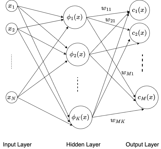
In the above RBF network, we use the weights connecting the input vector to hidden neurons to represent the center of that specific neuron. Further, we determine these weights in a manner such the receptive field of the hidden neurons covers the entire space. These are learned by someone other than training. We typically use K-means clustering on input $X$ to determine the hidden neurons’ weights (and center).

On the other hand, the weights connecting hidden neurons to output neurons are determined via training the network.

3.4. Training

RBF network training process involves two main steps:

Initialize the network
Apply gradient descent to learn model parameters (weights)

Our initialization phase involves applying K-means clustering on a subset of training data to determine the centroids of the hidden neurons. So, we determine the weights connecting the hidden layer to the output layer in the learning phase using a gradient descent algorithm. Further, we use mean square error (MSE) loss to model the error between the model output and ground truth output.

We choose $\sigma$ so that the receptive field of the hidden neurons covers the entire domain of input vector $X$ :

$\sigma = \frac{d}{\sqrt{2M}}$

In this formula, $d$ is the maximum distance between two hidden neurons, and $M$ is the total number of hidden neurons.

4. RBF vs MLP

Both these types of neural networks belong to the feed-forward network (FFN) class, but we use them for different use cases.

4.1. MLP

Like an RBF network, a multilayer perceptron (MLP ) is also an artificial neural network. To further elaborate, it is a fully connected neural network with a minimum of three layers. The first is an input layer. One or more hidden layers follow it, and finally, an output layer.

Internally, each MLP neuron uses a dot product between the input signal and connection weights. Then, it applies the sigmoid or ReLU activation function to generate the response. Further, an MLP network is trained through backpropagation for all layers in the network. We typically use MLP and other regularization techniques (dropout, batch normalization) to model a highly complex task.

4.2. MLP Use Case

MLPs outsmart RBFs in those cases where the underlying feature set is embedded deeply inside very high dimensional data sets.

For example, consider an image classification task. Here, the feature map depicting critical information about the image is hidden inside tens of thousands of pixels. So, this network requires training so that all the redundant features are filtered out as the image progresses through the network. Hence, we need a stack of hidden layers in MLPs for better performance.

However, the major drawback of such a network is that it takes longer to converge and requires significant computing and storage resources.

4.3. RBF Use Case

On the other side, RBFs have a single hidden layer. Thus, they have a much faster convergence rate than MLPs. This makes them an ideal candidate for processing low-dimensional datasets where we do not require deep feature extraction. Moreover, RBFs are very hard to approximate any complex function whose closed form is tedious to compute. So, in such cases, RBF acts as a robust learning model.

5. Conclusion

In this article, we have studied RBF.

RBF offers us several advantages. Primarily, it can approximate any continuous function to excellent precision precision. Secondly, it has a simple architecture and training process. More so, it offers fast convergence for a fairly high-dimensional dataset.

On the shadow side, RBFs may suffer from overfitting. A significant drawback is that they are sensitive to the number of centroids and their placement selection.

RBF networks provide a flexible and practical framework for solving various machine-learning tasks.

Full Archive

About Baeldung

Core Concepts

Operating Systems

Artificial Intelligence

Graph Theory

Latex