

Learn through the super-clean Baeldung Pro experience:
>> Membership and Baeldung Pro.
No ads, dark-mode and 6 months free of IntelliJ Idea Ultimate to start with.
Learn through the super-clean Baeldung Pro experience:
>> Membership and Baeldung Pro.
No ads, dark-mode and 6 months free of IntelliJ Idea Ultimate to start with.
In this tutorial, we’ll study the family of ReLU activation functions.
Before we dive into ReLU, let us talk about the activation function and its role in a generic neural network.
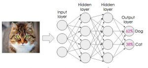
We define an artificial neural network as a higher-order mathematical model that we compose from interconnected nodes or artificial neurons. It mimics the structure and function of the human brain. For example, we can use it for information processing to solve complex problems such as image classification:
Moving on, our activation function is a mathematical function that a neuron executes. So, it calculates the output of a neuron as per its inputs and the associated weights on individual inputs.
It can be linear, such as unit function  , or non-linear such as the sigmoid function
  . Additionally, we also call these functions as the transfer functions:
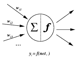
We typically use a non-linear activation function to solve complex real-world problems. This is so because most of these problems have complex relationships among their features.
Next, we move to artificial neural networks’ most common activation functions.
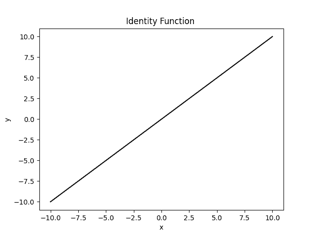
Identity function  is the most common linear activation. Its range is
  :
:
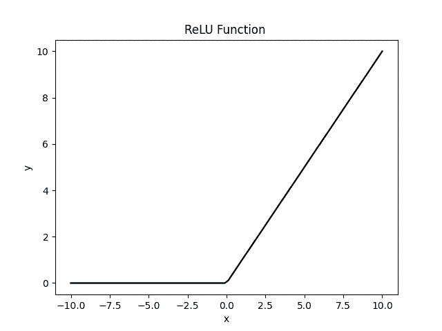
Among non-linear functions, ReLU is the most commonly used activation function. ReLU stands for rectified linear unit. Here,  when
when  and
and  when
when  . Further on, its range is
  :
:
The second most used non-linear activation function is the sigmoid function. We also call it the logistic activation function. To define, it takes input  and gives a value between
  . Therefore, we use it for models where we have to predict the probability as an output:
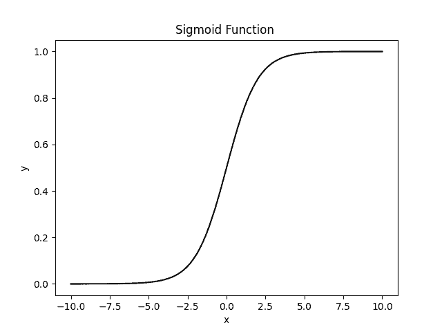
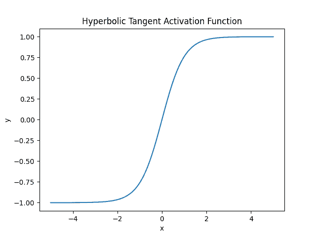
Another widespread non-linear activation is the tanh or hyperbolic tangent activation function. It works in the same way as the sigmoid. Further, the range of the tanh function is from  . It offers the advantage of mapping negative inputs to strictly negative output and mapping limiting zero inputs to near zero values in the tanh graph:
While training the model, the sigmoid and tanh activation suffer vanishing and exploding gradient problems (especially in hidden layers).
The vanishing gradient problem happens during training, whenever our gradients used to update the network become extremely small (vanish) during backpropagation from the output layers to the earlier layers. Thus, the weights need to be updated more to discover the underlying patterns in the data.
The exploding gradient problem occurs when our gradients become extremely large during the training process. As a result, model parameter weights get a significant update. Thus, this makes our model unstable, and continuing this way, it fails to learn all intractable patterns from our training data.
Apart from the above problems, we also have a few more. Both these functions are not centered around zero and thus are non-symmetric around the origin. Further, they are computationally expensive and have shallow slopes. Hence, they have low differentiability near the asymptotes, and thus, our training process takes longer.
In this section, we explore the ReLU function.
The basic version of Relu behaves as a unit function for positive inputs and 0 for negative inputs. Further, we find ReLU faster than sigmoid and tanh functions. Further, it doesn’t suffer from vanishing or exploding backpropagation errors.
However, it suffers from a dying-relu problem. ReLU makes all the negative input values zero immediately in the model graph. This makes the ReLU neuron inactive. We term this condition as the dead state of the ReLU neuron. It is challenging to recover in this state because the gradient 0 is 0. This problem is elevated when most of the training inputs are harmful, or the derivative of the ReLU function is 0.
We use Leaky ReLU to overcome this problem.
In this version, we use a slight non-negative gradient when the input is negative: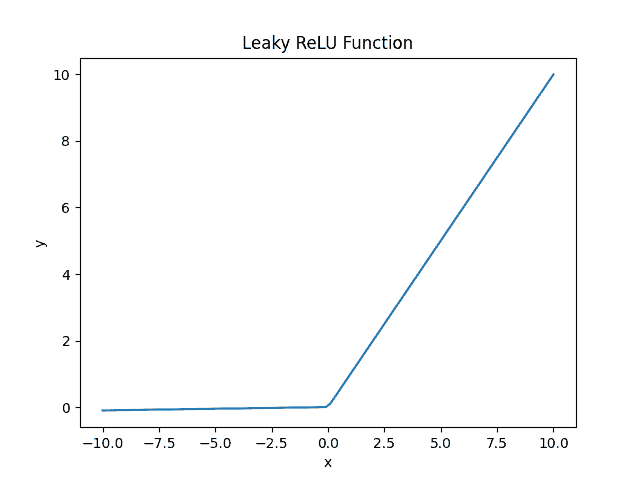
It allows small and non-zero gradients when the unit is inactive. This way, we overcame the dying real problem. However, it fails to give consistent predictions for negative inputs. It uses a slope  as a constant parameter throughout the training process. As the training values become more negative, their output becomes more and more linear. This way, we lose non-linearity at the cost of better gradient backpropagation.
Parametric ReLU or PReLU uses as a hyperparameter that the model learns during the training process: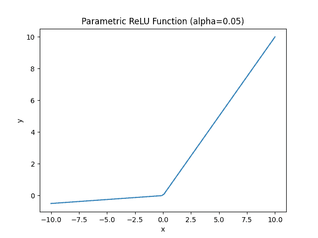
We use the PReLU activation function to overcome the shortcomings of ReLU and LeakyReLU activation functions. PReLU offers an increase in the accuracy of the model. Further, it gives us faster model convergence compared to LReLU and ReLU. However, it has one disadvantage. We must manually modify the parameter by trial and error. As you can see, this is a very time-consuming exercise, especially when our dataset is diverse.
, it outputs the product of with its Gaussian cumulative distribution function  . Going deeper, we find that the GeLU activation function scales inputs by their percentile, whereas the ReLU family of activation functions scales the inputs by their sign:
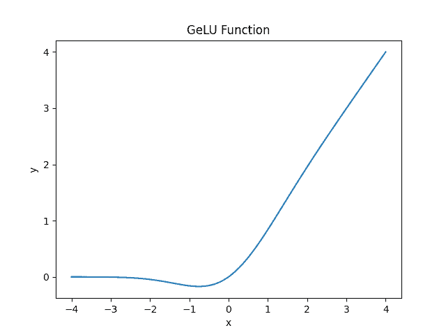
The following table summarizes the key differences between vanilla Relu and its two variants.
| Property | ReLU | LReLU | PReLU |
| Advantage | Solves gradient problems | Solves gradient problems | Solves gradient problems |
| Disadvantage | Dying relu problem | Inconsistent output for negative input | Fine-tune |
| Hyperparameter | None | None | 1 |
| Speed | Fastest | Faster | Fast |
| Accuracy | High | Higher | Highest |
| Convergence | Slow | Fast | Fastest |
In this article, we’ve gone through activation functions in an artificial neural network. After that, we delved into ReLU and its variants. ReLU is a simple yet powerful activation function that allows the neural network to learn intractable dependencies by introducing non-linearity. Moreover, its variants solve the gradient problems and give consistent output for negative input values.