Normalizing Inputs of Neural Networks | Baeldung on Computer Science

1. Introduction

Artificial neural networks are powerful methods for mapping unknown relationships in data and making predictions. One of the main areas of application is pattern recognition problems. It includes both classification and functional interpolation problems in general, and extrapolation problems, such as time series prediction.

Rarely, neural networks, as well as statistical methods in general, are applied directly to the raw data of a dataset. Normally, we need a preparation that aims to facilitate the network optimization process and maximize the probability of obtaining good results.

In this tutorial, we’ll take a look at some of these methods. They include normalization techniques, explicitly mentioned in the title of this tutorial, but also others such as standardization and rescaling.

We’ll use all these concepts in a more or less interchangeable way, and we’ll consider them collectively as normalization or preprocessing techniques.

2. Definitions

The different forms of preprocessing that we mentioned in the introduction have different advantages and purposes.

2.1. Normalization

Normalizing a vector (for example, a column in a dataset) consists of dividing data from the vector norm. Typically we use it to obtain the Euclidean distance of the vector equal to a certain predetermined value, through the transformation below, called min-max normalization:

$x'=\frac{x-x_{\min}}{x_{\max}-x_{\min}}(u-l)+l$

where:

$x$ is the original data.
$x'$ is the normalized data.
$x _ {\ max}, x _ {\ min}$ are respectively the maximum and minimum values of the original vector.
$u, l$ are respectively the upper and lower values of the new range for normalized data, $x ' \in [l: u]$ . Typical values are $[u = 1, l = 0]$ or $[u = 1, l = -1]$ .

The above equation is a linear transformation that maintains all the distance ratios of the original vector after normalization.

Some authors make a distinction between normalization and rescaling. The latter transformation is associated with changes in the unit of data, but we’ll consider it a form of normalization.

2.2. Standardization

Standardization consists of subtracting a quantity related to a measure of localization or distance and dividing by a measure of the scale. The best-known example is perhaps the called z-score or standard score:

$x'=\frac{x-\mu}{\sigma}$

where:

$\mu$ is the mean of the population.
$\sigma$ is the standard deviation of the population.

The z-score transforms the original data to obtain a new distribution with mean 0 and standard deviation 1.

Since generally we don’t know the values of these parameters for the whole population, we must use their sample counterparts:

$\hat{\mu}=\frac{1}{N}\sum_{i=1}^{N}x_{i}$

$\hat{\sigma}=\sqrt{\frac{1}{N-1}\sum_{i=1}^{N}(x_{i}-\hat{\mu})^{2}}$

where $N$ is the size of the vector $\mathbf {x}$ .

2.3. Batch Normalization

Another technique widely used in deep learning is batch normalization. Instead of normalizing only once before applying the neural network, the output of each level is normalized and used as input of the next level. This speeds up the convergence of the training process.

2.4. A Note on Usage

The application of the most suitable standardization technique implies a thorough study of the problem data. For example, if the dataset does not have a normal or more or less normal distribution for some feature, the z-score may not be the most suitable method.

The nature of the problem may recommend applying more than one preprocessing technique.

3. A Review on Normalization

Is it always necessary to apply a normalization or in general some form of data preprocessing before applying a neural network? We can give two responses to this question.

From a theoretical-formal point of view, the answer is: it depends. Depending on the data structure and the nature of the network we want to use, it may not be necessary.

Let’s take an example. Suppose we want to apply a linear rescaling, like the one seen in the previous section, and to use a network with linear form activation functions:

$y = w_ {0} + \sum_ {i = 1} ^ {N} w_ {i} x_ {i}$

where $y$ is the output of the network, $\mathbf {x}$ is the input vector with $N$ components $x_ {i}$ , and $w_ {i}$ are the components of the weight vector, with $w_ {0}$ the bias. In this case, normalization is not strictly necessary.

The reason lies in the fact that, in the case of linear activation functions, a change of scale of the input vector can be undone by choosing appropriate values of the vector $\mathbf {w}$ . If the training algorithm of the network is sufficiently efficient, it should theoretically find the optimal weights without the need for data normalization.

The second answer to the initial question comes from a practical point of view. In this case, the answer is: always normalize. The reasons are many and we’ll analyze them in the next sections.

3.1. Target Normalization

A neural network can have the most disparate structures. For example, some authors recommend the use of nonlinear activation functions for hidden level units and linear functions for output units. In this case, from the target point of view, we can make considerations similar to those of the previous section.

A widely used alternative is to use non-linear activation functions of the same type for all units in the network, including those of the output level. In this case, the output of each unit is given by a nonlinear transformation of the form:

$y = \mathcal {F} \left (w_ {0} + \sum_ {i = 1} ^ {N} w_ {i} x_ {i} \right)$

Commonly used functions are those belonging to the sigmoid family, such as those shown below, studied in our tutorial on nonlinear functions:

Common choices are the $\tanh$ , with image located in the range $[-1: 1]$ , or the logistic function, with image in the range $[0: 1]$ .

If we use non-linear activation functions such as these for network outputs, the target must be located in a range compatible with the values that make up the image of the function. By applying the linear normalization we saw above, we can situate the original data in an arbitrary range.

Many training algorithms explore some form of error gradient as a function of parameter variation. For example, the Delta rule, a form of gradient descent, takes the form:

$\Delta w = - \gamma \frac {\partial E} {\partial w}$

Due to the vanishing gradient problem, i.e. the cancellation of the gradient in the asymptotic zones of the activation functions, which can prevent an effective training process, it is possible to further limit the normalization interval. Typical ranges are $[-0.9: 0.9]$ for the $\tanh$ and $[0.1: 0.9]$ for the logistic function. Not all authors agree in the theoretical justification of this approach.

3.2. Input Normalization

As we have seen, the use of non-linear activation functions recommends the transformation of the original data for the target. However, there are also reasons for the normalization of the input.

The first reason, quite evident, is that for a dataset with multiple inputs we’ll generally have different scales for each of the features. We can make the same considerations for datasets with multiple targets. This situation could give rise to greater influence in the final results for some of the inputs, with an imbalance not due to the intrinsic nature of the data but simply to their original measurement scales. Normalizing all features in the same range avoids this type of problem.

Of course, if we have a priori information on the relative importance of the different inputs, we can decide to use customized normalization intervals for each. This is a possible but unlikely situation. In general, the relative importance of features is unknown except for a few problems.

Another reason that recommends input normalization is related to the gradient problem we mentioned in the previous section. The rescaling of the input within small ranges gives rise to even small weight values in general, and this makes the output of the units of the network near the saturation regions of the activation functions less likely. Furthermore, it allows us to set the initial range of variability of the weights in very narrow intervals, typically $[-1: 1]$ .

4. An Example

We applied a linear rescaling in the range $[- 1: 1]$ and a transformation with the z-score to the target of the abalone problem (number of rings), of the UCI repository. The characteristics of the original data and the two transformations are:

$\begin{array}{lcccc} \hline \mathrm{} & \mathrm{Mean} & \mathrm{Std.Dev} & \mathrm{Skewness} & \mathrm{Kurtosis}\\ \hline\hline \mathrm{Original\,data} & 9.934 & 3.2238 & 1.1137 & 5.3265\\ \mathrm{Normalization} & -0.3619 & 0.2303 & 1.1137 & 5.3265\\ \mathrm{z-score} & 1.364e-8 & 0.9999 & 1.1137 & 5.3265 \\\hline \end{array}$

with the distribution of the data after the application of the two transformations shown below:

Note that the transformations modify the individual points, but the statistical essence of the dataset remains unchanged, as evidenced by the constant values for skewness and kurtosis.

5. Standardization and Partitioning of the Dataset

5.1. Overview of the Problem

The analysis of the performance of a neural network follows a typical cross-validation process. The data are divided into two partitions, normally called a training set and test set. Most of the dataset makes up the training set. Typical proportions are $[0.67: 0.33]$ or $[0.75: 0.25]$ .

The process is as follows. The training with the algorithm that we have selected applies to the data of the training set. This process produces the optimal values of the weights and mathematical parameters of the network. The error estimate is however made on the test set, which provides an estimate of the generalization capabilities of the network on new data.

Between two networks that provide equivalent results on the test set, the one with the highest error in the training set is preferable. The unfamiliar reader in the application of neural networks may be surprised by this statement.

The reason lies in the fact that the generalization ability of an algorithm is a measure of its performance on new data. It can be empirically demonstrated that the more a network adheres to the training set, that is, the more effective it is in the interpolation of the single points, the more it is deficient in the interpolation on new partitions.

Some authors suggest dividing the dataset into three partitions: training set, validation set, and test set, with typical proportions $[0.50: 0.25: 0.25]$ . We measure the quality of the networks during the training process on the validation set, but the final results, which provide the generalization capabilities of the network, are measured on the test set. We can consider it a double cross-validation.

5.2. Preprocessing in Practice

Normalization should be applied to the training set, but we should apply the same scaling for the test data. That means storing the scale and offset used with our training data and using that again. A common beginner mistake is to separately normalize train and test data.

The reason should appear obvious. Normalization involves defining new units of measurement for the problem variables. We have to express each record, whether belonging to a training or test set, in the same units, which implies that we have to transform both with the same law.

The final results should consist of a statistical analysis of the results on the test set of at least three different partitions. This allows us to average the results of, particularly favorable or unfavorable partitions.

5.3. The Statistical Structure of the Dataset

Let’s go back to our main topic. For simplicity, we’ll consider the division into only two partitions. The considerations below apply to standardization techniques such as the z-score.

The general rule for preprocessing has already been stated above: in any normalization or preprocessing, do not use any information belonging to the test set in the training set. This criterion seems reasonable, but implicitly implies a difference in the basic statistical parameters of the two partitions.

This difference is due to empirical considerations, but not to theoretical reasons. It arises from the distinction between population and sample:

Considering the total of the training set and test set as a single problem generated by the same statistical law, we’ll not have to observe differences. In this situation, the normalization of the training set or the entire dataset must be substantially irrelevant.

Unfortunately, this is a possibility of purely theoretical interest. A case like this may be, in theory, if we have the whole population, that is, a very large number, at the infinite limit, of measurements.

In practice, however, we work with a sample of the population, which implies statistical differences between the two partitions. From an empirical point of view, it is equivalent to considering the two partitions generated by two different statistical laws.

In this case, the normalization of the entire dataset set introduces a part of the information of the test set into the training set. The data from this latter partition will not be completely unknown to the network, as desirable, distorting the end results.

All the above considerations, therefore, justify the rule set out above: during the normalization process, we must not pollute the training set with information from the test set.

The need for this rule is intuitively evident if we standardize the data with the z-score, which makes explicit use of the sample mean and standard deviation. But there are also problems with linear rescaling.

Suppose that we divide our dataset into a training set and a test set in a random way and that one or both of the following conditions occur for the target:

$t _ {\max} ^ {(train)} <t _ {\max} ^ {( test)$

$} t _ {\min} ^ {(train)}> t _ {\min} ^ {(test)}$

Suppose that our neural network uses $\tanh$ as the activation function for all units, with an image in the interval $[-1: 1]$ . We’re forced to normalize the data in this range so that the range of variability of the target is compatible with the output of the $\tanh$ . However, if we normalize only the training set, a portion of the data for the target in the test set will be outside this range.

For these data, it will, therefore, be impossible to find good approximations. If the partitioning is particularly unfavorable and the fraction of data out of the range $[-1: 1]$ is large, we can find a high error for the whole test set.

5.5. Possible Solutions of the Problem

We can try to solve the problem in several ways:

We narrow the normalization interval of the training set, to have the certainty that the entire dataset is within the range . This approach does not completely solve the problem:
- Part of the test set data may fall into the asymptotic areas of the activation function. These records may be susceptible to the vanishing gradient problem.
- Training will be effective only in the $\tanh$ image regions covered by the training set data. The network will be forced to perform extrapolation instead of interpolation, which is generally a simpler problem.
In the case of linear rescaling, which maintains distance relationships in the data, we may decide to normalize the whole dataset. This is equivalent to the point above.
The best approach in general, both for normalization and standardization, is to achieve a sufficiently large number of partitions. This approach smoothes out the aberrations highlighted in the previous subsections.

6. Power Transforms

Neural networks can be designed to solve many types of problems. They can directly map inputs and targets but are sometimes used to obtain the optimal parameters of a model.

Many models in the sciences make use of Gaussian distributions. The assumption of the normality of a model may not be adequately represented in a dataset of empirical data. Situations of this type can be derived from the incompleteness of the data in the representation of the problem or the presence of high noise levels.

In these cases, it is possible to bring the original data closer to the assumptions of the problem by carrying out a monotonic or power transform. The result is a new more normal distribution-like dataset, with modified skewness and kurtosis values. We can consider it a form of standardization.

We’ll study the transformations of Box-Cox and Yeo-Johnson.

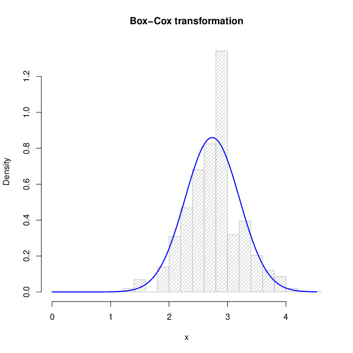
6.1. Box-Cox Transform

The transformation of Box-Cox to a parameter is given by:

$x_ {i} ^ {(\lambda)} = \left \ {\begin {array} {ll} \frac {x_ {i} ^ {\lambda} -1} {\lambda}, & \lambda \neq0 \\ \ln x_ {i}, & \lambda = 0 \end {array} \right$

$\lambda$ is the value that maximizes the logarithm of the likelihood function:

$\ln \mathcal {L} = - \frac {N} {2} \ln \sigma ^ {2} + (\lambda-1) \sum_ {i = 1} ^ {N} \ln x_ {i}$

The presence of the logarithm prevents the application to datasets with negative values. In this case a rescaling on positive data or the use of the two parameter version is necessary:

$x_ {i} ^ {(\lambda_ {1}, \lambda_ {2})} = \left \ {\begin {array} {ll} \frac {(x_ {i} + \lambda_ {2}) ^ {\lambda_ {1}} - 1} {\lambda}, & \lambda_ {1} \neq0 \\ \ln (x_ {i} + \lambda_ {2}), & \lambda_ {1} = 0 \End {array} \right$

6.2. Yeo-Johnson Transform

The Yeo-Johnson transformation is given by:

$x_ {i} ^ {(\lambda)} = \left \ {\begin {array} {ll} \frac {\left (x_ {i} +1 \ right) ^ {\lambda} -1} {\lambda}, & \lambda \neq0, x_ {i} \geq0 \\ \ln (x_ {i} +1), & \lambda = 0, x_ {i} \geq0 \\ - \frac {(- x_ {i} +1) ^ {2- \lambda} -1} {2- \lambda}, & \lambda \neq2, x_ {i} <0 \\ - \ln (-x_ {i} +1), & \lambda = 2, x_ {i} <0 \end {array} \right$

Yeo-Johnson’s transformation solves a few problems with Box-Cox’s transformation and has fewer limitations when applying to negative datasets.

Both methods can be followed by linear rescaling, which allows preserving the transformation and adapt the domain to the output of an arbitrary activation function.

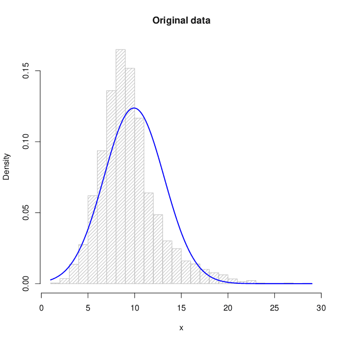
7. A Real Example

We applied both transformations to the target of the abalone problem (number of rings), of the UCI repository. The distribution of the original data is:

For Box-Cox transform:

For Yeo-Johnson transform:

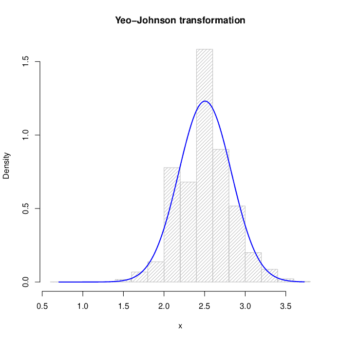
The numerical results before and after the transformations are in the table below. The reference for normality is skewness $= 0$ and kurtosis $= 0$ :

$\begin{array}{lcc} \hline \mathrm{} & \mathrm{Skewness} & \mathrm{Kurtosis}\\ \hline\hline \mathrm{Original\,data} & 1.1137 & 5.3265\\ \mathrm{Box-Cox} & 0.0183 & 0.9733\\ \mathrm{Yeo-Johnson} & 0.0044 & 0.8648 \\\hline \end{array}$

8. Conclusions

In this tutorial, we took a look at a number of data preprocessing and normalization techniques. The quality of the results depends on the quality of the algorithms, but also on the care taken in preparing the data. We have given some arguments and problems that can arise if this process is carried out superficially.

There are other forms of preprocessing that do not fall strictly into the category of “standardization techniques” but which in some cases become indispensable. The Principal Component Analysis (PCA), for example, allows us to reduce the size of the dataset (number of features) by keeping most of the information from the original dataset or, in other words, by losing a certain amount of information in a controlled form.

PCA and other similar techniques allow the application of neural networks to problems susceptible to an aberration known under the name of the curse of dimensionality, i.e. the provision of an insufficient amount of data to be able to identify all decision boundaries in high-dimensional problems.

Full Archive

About Baeldung

Core Concepts

Operating Systems

Artificial Intelligence

Graph Theory

Latex