What the Correlation Coefficient Actually Represents

1. Overview

In this tutorial, we’ll study the meaning of the correlation coefficient in the correlation analysis.

We’ll first start by discussing the idea of correlation in general between variables. This will help us understand why correlation analysis was developed in the first place.

Then, we’ll learn the two main techniques for correlation analysis, Spearman and Pearson’s correlation. In relation to them, we’ll see both the mathematical formulation and their applications.

Lastly, we’ll make a summary of what we can infer about a bivariate distribution on the basis of the values of its correlation coefficients.

At the end of this tutorial, we’ll have an intuitive understanding of what the correlation coefficients represent. We’ll also be able to choose between the Spearman and Pearson correlation, in order to solve concrete tasks we’re facing.

2. Correlation in General

2.1. The Idea of Correlation

Correlation analysis is a methodology for statistical analysis, dedicated to the study of the relationship between random variables. It’s also sometimes called dependence because it relates to the idea that the value of one variable might depend on another. We’re soon going to study the mathematical definition of correlation. But first, it’s better to get a general idea of what correlation means intuitively.

We can do so with a small example. We know that, in general, the weight and height of an individual tend to go together. This means that the taller a person is, the higher their weight tends to be:

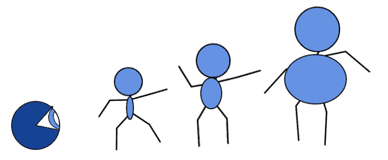
This leads us to hypothesize that the relationship between weight and height might be characterized by dependence. In order to test this hypothesis, though, we need some kind of measure or index for the degree of dependence between two variables. That measure is what we call correlation.

We might, in fact, imagine that the relationship of dependence can either be strong or weak or simply be completely absent:

The index we need should let us distinguish at a glance between those cases, on the basis of the value that it possesses.

2.2. Correlation and Not Causation

Correlation is an important tool in exploratory data analysis because it allows the preliminary identification of features that we suspect to not be linearly independent. It’s also important in the identification of causal relationships because there are known methodologies for testing causality that use correlation as to their core metric.

There’s a common sentence among statisticians which says that correlation doesn’t imply causation. The idea behind this is that, for two variables that are correlated, a relationship of causality can’t be given for granted.

The implication to which we refer here is the so-called material implication in propositional logic. We can, therefore, use the rules for working with implications in order to formalize its expression. If $r$ identifies correlation, and $c$ identifies causation, then this implication formally states that $\neg (r \to c)$ .

We studied in our article on Boolean logic that we can rewrite an expression of the form $p \to q$ as $\neg p \vee q$ . This means that we can convert the expression $\neg (r \to c)$ to $\neg (\neg r \vee c)$ . If we use De Morgan’s law on the terms between brackets, we then obtain $r \wedge \neg c$ , which is true if there is a correlation but there isn’t causation.

2.3. When Does Correlation Not Imply Causation?

There are some common logical mistakes that may lead us to think that there’s causation among two variables as a consequence of the observed correlation. These mistakes take the name of fallacies and frequently lead to the wrong understanding of what correlation actually represents.

The first argument corresponds to the incorrect identification of the variable that causes the other.

If $p$ and $q$ are variables about which we test their causal relationship, and if the true causal relationship has the form $p \to q$ while simultaneously implying a high correlation $r_{p \to q}$ , then $r_{q \to p}$ will also be necessarily high. This means that we might incorrectly end up identifying $q$ as the cause and $p$ as the consequence of the causal relationship, and not the other way around.

An example of this might be the following. We noted a strange behavior. Immediately upon putting food into a bowl, a cat comes, meows, and eats it:

We might be tempted to infer that the filling of the bowl causes a cat to appear since the correlation between these events would be very high. In this case, though, we would be surprised if, not owning a cat, a cat fails to appear after we fill a bowl:

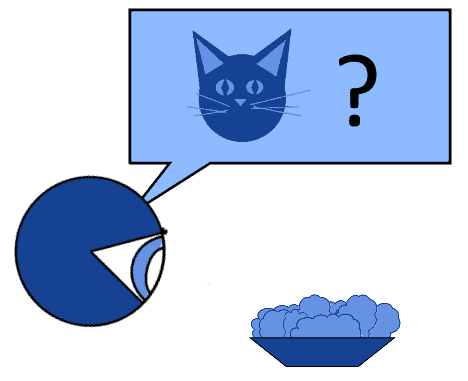
In this example, we are incorrectly assigning antecedence in the relation of causality to the filling of the bowl. Instead, we should assign it to the presence of the cat, which causes us to fill the bowl in reaction to its presence.

2.4. A Third Factor

A second argument relates to the incorrect inference of a relationship of causality between two events that are, both, consequences of a third unseen event $s$ . This corresponds, with formal notation, to the expression $(s \to p) \wedge (s \to q)$ . The classic example for this argument corresponds to the relationship between the arrival of passengers and that of a train to a platform in a train station:

If we knew nothing about timetables and their operation, we might end up thinking that the arrival of passengers causes the train to appear. In reality, though, a third factor, the scheduling of the passenger train, causes both the passengers and the train to appear at the appointed time.

2.5. Causation and Not Correlation

A less frequently discussed question is whether the presence of a causal relationship between an independent and a dependent variable also implies correlation. With formal notation, we can express this question with the proposition $c \to r$ .

There certainly are causally-dependent variables that are also correlated to one another. In the sector of pharmacology, for example, the research on adverse drug reactions developed extensive methodologies for assessing causality between correlated variables. In the sector of pedagogy and education, similar methods also exist to assess causality between correlated variables, such as family income and student performances.

As a general rule, however, causality doesn’t imply correlation. This is because correlation, especially Pearson’s as we’ll see shortly, measures only one type of functional relationship: linear relationships. While Spearman’s correlation fares slightly better, as we’ll see soon, it still fails to identify non-monotonic relationships between variables:

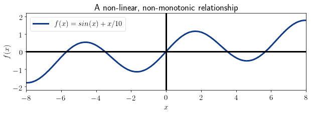
This means that, as a general rule, we can infer correlation from causality only for linear or monotonic relationships.

3. Pearson’s Correlation Coefficient

3.1. Introduction to Pearson Correlation

We can now get into the study of the two main techniques for calculating the correlation between variables: Pearson and Spearman’s correlations.

Pearson’s correlation is the oldest method for calculating dependence between random variables, and it dates back to the end of the 19th century. It’s based upon the idea that a linear regression model may fit a bivariate distribution with varying degrees of accuracy. Pearson’s correlation thus provides a way to assess the fit of a linear regression model.

It’s also invariant under scaling and translation. This means that Pearson’s correlation is particularly useful for studying the properties of hierarchical or fractal systems, which are scale-free by definition.

3.2. Mathematical Definition of Pearson’s Correlation

We can define the Pearson’s correlation coefficient $r_{xy}$ between two random variables $x$ and $y$ with $k$ components as the covariance of $x$ and $y$ , divided by the product of their respective standard deviations:

$r_{xy} = \frac{ \sum_{i=1}^{k} (x_i - \overline{x}) (y_i - \overline{y}) } { \sqrt { \sum_{i=1}^{k} (x_i - \overline{x})^2 } \sqrt { \sum_{i=1}^{k} (y_i - \overline{y})^2 } }$

In here, $\overline{x}$ and $\overline{y}$ indicate the averages of the two variables. The correlation coefficient $r_{xy}$ assumes a value in the closed interval $[-1, 1]$ , where $r_{xy} = 1$ indicates maximum positive correlation, $r_{xy} = 0$ corresponds to lack of correlation, and $r_{xy} = -1$ denotes maximum negative correlation.

In our article on linear regression, we also studied the relationship between this formula and the regression coefficient, which provides another way to compute the same correlation coefficient.

3.3. Possible Values

We’re now going to study the possible values that the correlation coefficient can assume, and observe the shape of the distributions that are associated with each value.

For $r_{xy} \cong 0$ , the two variables are uncorrelated. This means that the value assumed by one variable generally doesn’t influence the value assumed by the other:

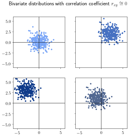
Uncorrelated bivariate distributions generally, but not necessarily, assume their typical “cloud” shape. If we spot this shape when plotting a dataset, we should immediately suspect that the distribution isn’t correlated.

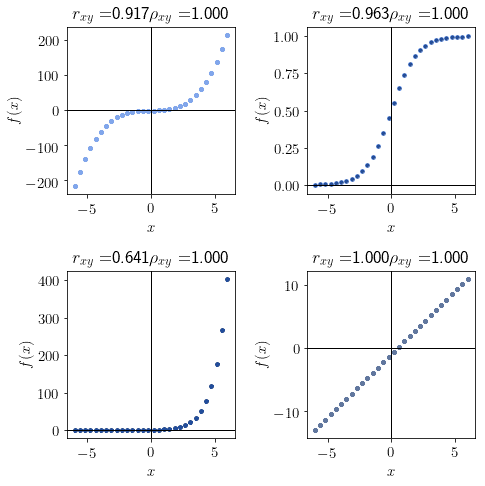
For $r_{xy} = 1$ , the variables are strongly positively correlated. Any bivariate distribution that can be fitted perfectly by a linear regression model with a positive slope always has a correlation coefficient of 1:

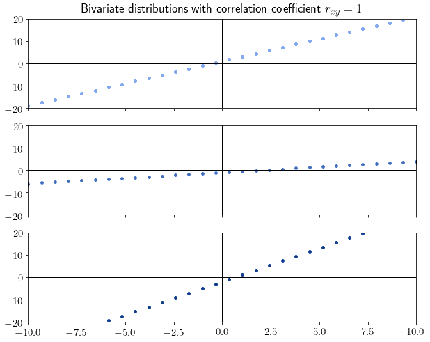
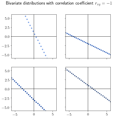
Intuitively, if we see that the distribution assumes the shape of a line, we should now that the absolute value of the correlation is high. The sign of the slope, then, determines the sign of the correlation. For this reason, the correlation value of $r_{xy} = -1$ implies a linear distribution with negative slope:

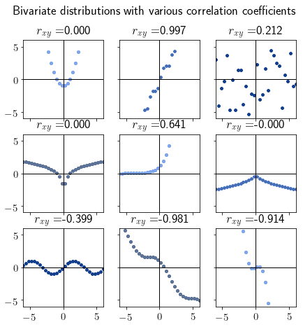
Most distributions don’t however have a perfect correlation value of 0, or $\pm$ 1. They do however tend to either a cloud or line-shaped functions, respectively, as the correlation approximates them. Here are some other examples of distributions with the respective correlation coefficients:

3.4. Interpretation of Pearson’s Correlation Coefficient

There’s a typical mistake that many make in interpreting the Pearson correlation coefficient. This mistake consists of reading it as the slope of the linear regression model that best fits the distribution. The pictures above show that, for variables that span a line perfectly, the correlation coefficient is always $\pm$ 1 regardless of that line’s slope. This means that the correlation coefficient isn’t the slope of a line.

It is, however, a good predictor of how well a linear regression model would fit the distribution. In the extreme case of $r_{xy} = \pm 1$ , a linear regression model would fit perfectly the data with an error of 0. In the extreme case of $r_{xy} = 0$ , no linear regression model will fit the distribution well.

4. Spearman’s Rank Correlation

4.1. Introduction to Spearman

A more refined measure for determining correlation is the so-called Spearman rank correlation. This correlation is normally indicated with the symbol $\rho_{xy}$ and can assume any values in the interval $[-1,1]$ , like Pearson’s.

This correlation coefficient was developed to obviate a problem that Pearson’s correlation possesses. When considering distributions that are strongly monotonic, Pearson’s coefficient doesn’t necessarily correspond to $\pm 1$ :

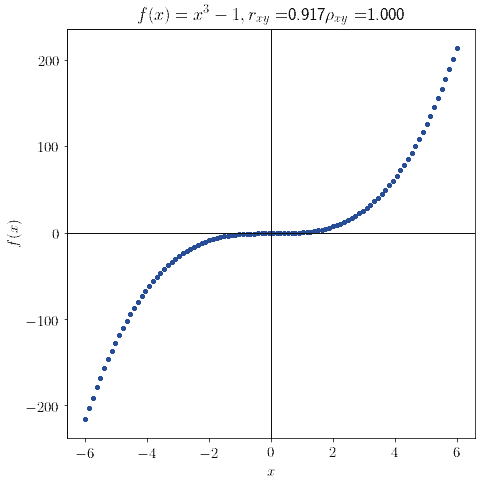
Spearman’s coefficient solves this problem, allowing to identify monotonicity in general, and not only in the specific case of linearity in the bivariate distribution.

4.2. Mathematical Definition of Pearson’s Correlation

Unlike Pearson’s coefficient, $\rho_{xy}$ is non-parametric and is calculated on ranks rather than on the variables themselves. The rank of a variable consists of the replacement of its values with the position that that particular value occupies in the sorted variable. If, for example, we want to calculate the rank $rg_x$ of $x = [5.3, 2.8, 4.2, 3, 1.4]$ , we should first $x$ as $[1.4, 2.8, 3, 4.2, 5.3]$ . The rank is then computed by replacing each original value of the variable with its position in the sorted one, as $rg_x = [5, 2, 4, 3, 1]$ .

The Spearman correlation coefficient of $\rho_{xy}$ is then calculated as:

$\rho_{xy} = \frac {\text{cov}(rg_x, rg_y)} {\sigma(rg_x) \sigma(rg_y)}$

where $\text{cov}(rg_x, rg_y)$ is the covariance of $rg_x, rg_y$ and $\sigma(rg_x) \sigma(rg_y)$ is the product of the two respective standard deviations.

4.3. Possible Values

As anticipated earlier, the Spearman coefficient varies between -1 and 1. For $\rho_xy = 1$ , the bivariate distribution is monotonically increasing:

Similarly, a distribution with a Spearman coefficient $\rho_{xy} = -1$ is monotonically decreasing:

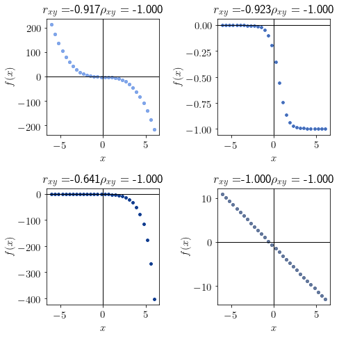
And lastly, a value of $rho_{xy} \cong 0$ indicates that a function isn’t monotonic:

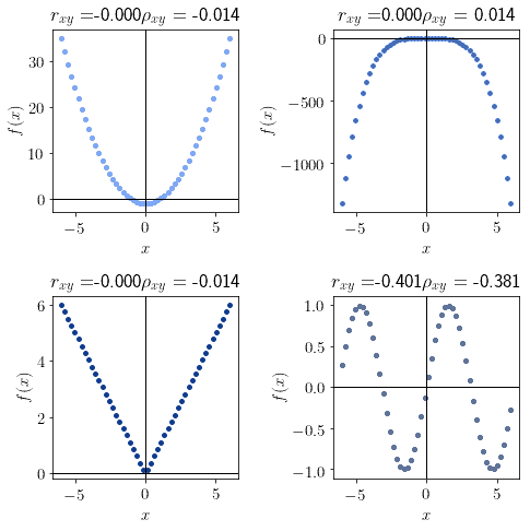
Notice that all distributions sampled from even functions of the form $f(x) = f(-x)$ have a Spearman correlation coefficient $\rho_{x, f(x)} = 0$ .

4.4. Interpretation of Spearman’s Correlation Coefficient

We can finally discuss the interpretation of the value assumed by the Spearman correlation coefficient in a more formal manner. We saw earlier that it relates to monotonicity. Therefore, if we have a distribution sampled from a function of the form $y = f(x)$ , the sign of $\rho_{xy}$ points, in general, at the tonicity of that function.

Spearman doesn’t however only apply to functionally dependent variables, since we can use it for all random variables. As a consequence, we need a definition that doesn’t rely on concepts taken from the analysis of continuous functions.

Rather, we can interpret it as the degree by which two variables tend to change in the same direction. That is to say, variables with high correlation all increase and decrease simultaneously, while variables with low absolute correlation rarely decrease together. In other words, the correlation coefficient tells us, for any difference $\Delta{x} = x_i - x_j$ between two components of $x$ , the sign of the corresponding difference $\Delta{y} = y_i - y_j$ .

In this sense, a correlation $\rho_{xy} = 1$ tells us that $(\Delta{x} \geq 0 \to \Delta{y} \geq 0) \wedge (\Delta{x} \leq 0 \to \Delta{y} \leq 0)$ . Similarly, a coefficient $\rho_{xy}=-1$ implies $(\Delta{x} \geq 0 \to \Delta{y} \leq 0) \wedge (\Delta{x} \leq 0 \to \Delta{y} \geq 0)$ . And lastly, a correlation coefficient $\rho_{xy}=-0$ means that neither of the previous expressions are true.

5. Interpretation of the Two Coefficients

5.1. The Values of the Correlation Coefficients

We can now sum up the considerations made above and create a table containing the theoretical prediction that we can make about a bivariate distribution according to the values of its correlation coefficients:

5.2. Guessing Correlation Values

We’re now going to use this table to conduct the inverse process. That is, to guess the correlation value of distributions on the basis of their shape. This can be helpful to formulate hypotheses on their values, which we can then test computationally. We do so by observing the shape of the distribution, compare it with the table we drafted above, and then infer the probable values of the correlation coefficients.

The first distribution is this:

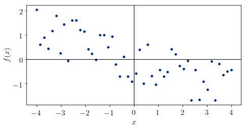
We can note that it looks vaguely shaped as a linear function, and that it’s generally decreasing. For this reason, we expect its $r_{xy}$ and $\rho_{xy}$ values to be comprised in the interval $r_{xy}, \rho_{xy} \in (-1,0)$ . The real values for this distribution are $r_{xy} = -0.734$ and $\rho_{xy} = -0.721$ , which means that our guess was correct.

The second variable has a shape that resembles the logistic function $y =\sigma(x)$ :

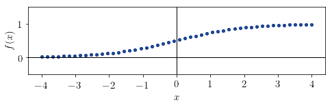
Because it’s monotonically increasing, its $\rho_{xy}$ value must be +1. It also seems that it doesn’t fit perfectly into a line but is generally approximable with a linear model. From this we derive that its $r_{xy}$ value must be in the interval $(0, +1)$ . The true values of the coefficients for this distribution are $r_{xy} = 0.982$ and $\rho_{xy} = 1$ , which means that we guessed correctly.

The third distribution has the shape of a sinusoidal:

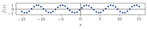
The function can’t be monotonic, and it doesn’t seem to be increasing or decreasing. This means that the Spearman coefficient $\rho_{xy}$ is approximately 0. It also doesn’t seem approximable by a linear model, which means that it’s Pearson coefficient should be close to 0, too. The real values for this distribution are $r_{xy} = 0.152$ and $\rho_{xy} = 0.144$ , which are indeed close enough to 0, as we expected.

6. Conclusions

In this article, we studied the concept of correlation for bivariate distributions.

We first approached the issue of the relationship between correlation and causality.

Then, we studied Pearson’s correlation and its interpretation, and similarly Spearman’s correlation.

In doing so, we learned that Pearson’s correlation relates to the suitability of the distribution for linear regression. Spearman’s coefficient, instead, relates to the monotonicity of a continuous function that would approximate the distribution.

Full Archive

About Baeldung

Core Concepts

Operating Systems

Artificial Intelligence

Graph Theory

Latex