

Yes, we're now running our only Summer Sale. All Courses are 30% off until 20th July, 2026:
What Is Inductive Bias in Machine Learning?
Last updated: February 13, 2025
Learn through the super-clean Baeldung Pro experience:
>> Membership and Baeldung Pro.
No ads, dark-mode and 6 months free of IntelliJ Idea Ultimate to start with.
1. Overview
In this tutorial, we’ll discuss a definition of inductive bias and go over its different forms in machine learning and deep learning.
2. Definition
Every machine learning model requires some type of architecture design and possibly some initial assumptions about the data we want to analyze. Generally, every building block and every belief that we make about the data is a form of inductive bias.
Inductive biases play an important role in the ability of machine learning models to generalize to the unseen data. A strong inductive bias can lead our model to converge to the global optimum. On the other hand, a weak inductive bias can cause the model to find only the local optima and be greatly affected by random changes in the initial states.
We can categorize inductive biases into two different groups called relational and non-relational. The former represents the relationship between entities in the network, while the latter is a set of techniques that further constrain the learning algorithm.
3. Inductive Biases in Machine Learning
In traditional machine learning, every algorithm has its own inductive biases. In this section, we mention some of these algorithms.
3.1. Bayesian Models
Inductive bias in Bayesian models shows itself in the form of the prior distributions that we choose for the variables. Consequently, the prior can shape the posterior distribution in a way that the latter can turn out to be a similar distribution to the former. In addition, we assume that the variables are conditionally independent, meaning that given the parents of a node in the network, it’ll be independent from its ancestors. As a result, we can make use of conditional probability to make the inference. Also, the structure of the Bayesian net can facilitate the analysis of causal relationships between entities.
3.2. k-Nearest Neighbors (k-NN) Algorithm
The k-Nearest Neighbors ( ) algorithm assumes that entities belonging to a particular category should appear near each other, and those that are part of different groups should be distant. In other words, we assume that similar data points are clustered near each other away from the dissimilar ones.
3.3. Linear Regression
Given the ( ,
,  ) data points, in linear regression, we assume that the variable () is linearly dependent on the explanatory variables (). Therefore, the resulting model linearly fits the training data. However, this assumption can limit the model’s capacity to learn non-linear functions.
3.4. Logistic Regression
In logistic regression, we assume that there’s a hyperplane that separates the two classes from each other. This simplifies the problem, but one can imagine that if the assumption is not valid, we won’t have a good model.
4. Relational Inductive Biases in Deep Learning
Relational inductive biases define the structure of the relationships between different entities or parts in our model. These relations can be arbitrary, sequential, local, and so on.
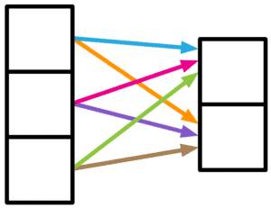
4.1. Weak Relation
Sometimes the relationship between the neural units is weak, meaning that they’re somewhat independent of each other. The choice of including a fully connected layer in the net can represent this kind of relationship:
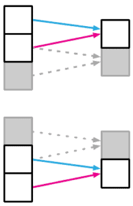
4.2. Locality
In order to process an image, we start by capturing the local information. One way to do that is the use of a convolutional layer. It can capture the local relationship between the pixels of an image. Then, as we go deeper in the model, the local feature extractors help to extract the global features:
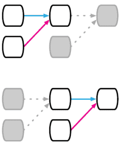
4.3. Sequential Relation
Sometimes our data has a sequential characteristic. For instance, time series and sentences consist of sequential elements that appear one after another. To model this pattern, we can introduce a recurrent layer to our network:
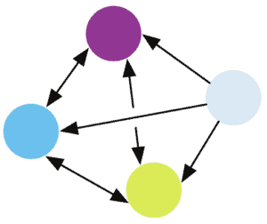
4.4. Arbitrary Relation
To solve problems related to a group of things or people, it might be more informative to see them as a graph. The graph structure imposes arbitrary relationships between the entities, which is ideal when there’s no clear sequential or local relation in the model:
5. Non-Relational Inductive Biases in Deep Learning
Other than relational inductive biases, there are also some concepts that impose additional constraints on our model. In this section, we list some of these concepts.
5.1. Non-linear Activation Functions
Non-linear activation functions allow the model to capture the non-linearity hidden in the data. Without them, a deep neural network wouldn’t be able to work better than a single-layer network. The reason is that the combination of several linear layers would still be a linear layer.
5.2. Dropout
Dropout is a regularization technique that helps the network avoid memorizing the data by forcing random subsets of the network to each learn the data pattern. As a result, the obtained model, in the end, is able to generalize better and avoid overfitting.
5.3. Weight Decay
Weight decay is another regularization method that puts constraints on the model’s weights. There are several versions of weight decay, but the common ones are  and
and  regularization techniques. Weight decay doesn’t let the weights grow very large, which prevents the model from overfitting.
5.4. Normalization
Normalization techniques can help our model in several ways, such as making the training faster and regularizing. But most importantly, it reduces the change in the distribution of the net’s activations which is called internal co-variate shift. There are different normalization techniques such as batch normalization, instance normalization, and layer normalization.
5.5. Data Augmentation
We can think of data augmentation as another regularization method. What it imposes on the model depends on its algorithm. For instance, adding noise or word substitution in sentences are two types of data augmentation. They assume that the addition of the noise or word substitution should not change the category of a sequence of words in a classification task.
5.6. Optimization Algorithm
The optimization algorithm has a key role in the model’s outcome we want to learn. For example, different versions of the gradient descent algorithm can lead to different optima. Subsequently, the resulting models will have other generalization properties. Moreover, each optimization algorithm has its own parameters that can greatly influence the convergence and optimality of the model.
6. Conclusion
In this tutorial, we learned about the two types of inductive biases in traditional machine learning and deep learning. In addition, we went through a list of examples for each type and explained the effects of the given examples.