Instance vs Batch Normalization | Baeldung on Computer Science

1. Overview

This tutorial will go over two normalization techniques in deep learning, namely Instance Normalization (IN) and Batch Normalization (BN). We’ll also highlight the differences between these two methods.

2. Motivation for Normalization

Let’s start with the reason for performing normalization in deep neural nets. Normalization or feature scaling is a way to make sure that features with very diverse ranges will proportionally impact the network performance. Without normalization, some features or variables might be ignored.

For example, imagine that we want to predict the price of a car using two features such as the driven distance and the car’s age. The first feature’s range is in thousands whereas the second one is in the range of tens of years. Using the raw data for predicting the price of the car, the distance feature would outweigh the age feature significantly. Therefore, we should normalize these two features to get a more accurate prediction.

For a more detailed discussion on the concept of normalization and its variants, see Normalizing Inputs for an Artificial Neural Network.

Usually, normalization is carried out in the input layer to normalize the raw data. However, for deep neural nets, the activation values of the middle layer nodes can get very large, causing the same problem as our example. This necessitates some type of normalization in the hidden layers as well.

3. Instance Normalization (IN)

Instance normalization is another term for contrast normalization, which was first coined in the StyleNet paper. Both names reveal some information about this technique. Instance normalization tells us that it operates on a single sample. On the other hand, contrast normalization says that it normalizes the contrast between the spatial elements of a sample. Given a Convolution Neural Network (CNN), we can also say that IN performs intensity normalization across the width and height of a single feature map of a single example.

To clarify how IN works, let’s consider sample feature maps that constitute an input tensor to the IN layer. Let $x$ be that tensor consisting of a batch of $N$ images. Each of these images has $C$ feature maps or channels with height $H$ and weight $W$ . Therefore, $x \in \R^{N\times C\times H\times W}$ is a four-dimensional tensor. In instance normalization, we consider one training sample and feature map (specified in red in the figure) and take the mean and variance over its spatial locations ( $W$ and $H$ ):

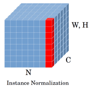
To perform instance normalization for a single instance $x_{ni}$ , we need to compute the mean and variance:

$\mu_{ni} = \frac{1}{HW} \sum_{l=1}^{W} \sum_{m=1}^{H} x_{nilm}$

$\sigma^2_{ni} = \frac{1}{HW} \sum_{l=1}^{W} \sum_{m=1}^{H} (x_{nilm} - \mu_{ni})^2$

Then, using the obtained mean and variance, each spatial dimension is normalized:

$y_{nijk} = \frac{x_{nijk} - \mu_{ni}}{\sqrt{\sigma^2_{ni} + \epsilon}}$

where $\epsilon$ is a small value added for more stable training. In the end, using two scaling and bias parameters, we linearly transform the result. This transformation preserves the network’s capacity by ensuring that the normalization layer can produce the identity function. The network learns the two parameters during training. For instance, to obtain the identity function, if needed, the network will learn that $\gamma = \sqrt{\sigma^2_{ni} + \epsilon}}$ and $\beta = \mu_{ni}$ .

4. Batch Normalization (BN)

Considering the same feature maps of the previous figure, BN operates on one channel (one feature map) over all the training samples in the mini-batch (specified in red):

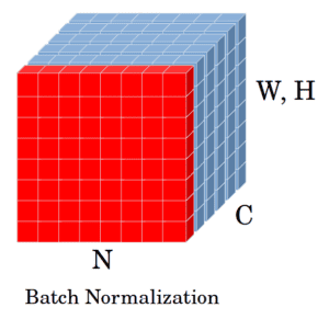
Let $B = \{x_1, x_2, ..., x_N\}$ be a mini-batch of size $N$ . BN normalizes its activation values using the mean ( $\pmb{\mu_i}$ ) and variance ( $\pmb{\sigma^2_i}$ ) of the mini-batch and introduces two learnable parameters, $\gamma$ and $\beta$ . The network can learn these parameters using a Gradient Descent algorithm.

$\mu_{i} = \frac{1}{NHW} \sum_{n=1}^{N} \sum_{l=1}^{W} \sum_{m=1}^{H} x_{nilm}$

$\sigma^2_{i} = \frac{1}{NHW} \sum_{n=1}^{N} \sum_{l=1}^{W} \sum_{m=1}^{H} (x_{nilm} - \mu_i)^2$

Similar to IN, we add the $\epsilon$ in computing $\hat{x}_{nijk}$ to the denominator to stabilize the training in case the variance of the mini-batch is zero.

$\hat{x}_{nijk} = \frac{x_{nijk} - \mu_i}{\sqrt{\sigma^2_i + \epsilon}}$

Finally,

$y_{nijk} = \gamma \hat{x}_{nijk} + \beta$

The $\gamma$ and $\beta$ parameters are the same as the scaling and bias operators of IN and have the same functionality.

5. Understanding the Differences Between IN and BN

Both normalization methods can accelerate training and make the network converge faster. Plus, BN enables larger training rates and improves the generalization of the neural network. Having said that, there are several differences between these two forms.

First of all, based on their definition, they function differently on their inputs. While IN transforms a single training sample, BN does that to the whole mini-batch of samples. This makes BN dependent on the batch size in that, to obtain a statistically more accurate mean and variance, the batch size needs to be large.

However, this can be difficult to implement since a large batch size requires large memory. As a result, when we have a limitation on the memory, we’ll have to opt for smaller batch sizes which can be problematic in some cases. Using a very small batch size can introduce error to the training because the mean and variance become noisier. A small batch size setting is where IN performs better than BN.

In addition, since BN is dependent on the batch size, it can’t be applied at test time the same way as the training time. The reason is that in the test phase, we usually have one example to process. Therefore, the mean and variance can’t be computed like training. Instead, during test time, BN utilizes moving average and variance to perform inference. In contrast, IN doesn’t depend on the batch size, so its implementation is kept the same for both training and testing.

6. Conclusion

In this tutorial, we described how instance and batch normalization methods work. We also pointed out the major differences between the two norms in terms of implementation and use cases.

Full Archive

About Baeldung

Core Concepts

Operating Systems

Artificial Intelligence

Graph Theory

Latex