

Learn through the super-clean Baeldung Pro experience:
>> Membership and Baeldung Pro.
No ads, dark-mode and 6 months free of IntelliJ Idea Ultimate to start with.
Learn through the super-clean Baeldung Pro experience:
>> Membership and Baeldung Pro.
No ads, dark-mode and 6 months free of IntelliJ Idea Ultimate to start with.
Every day, numerous events happen because of one or several reasons. After observing an event, as curious human beings, we’d like to understand the reason why something happened in its particular form. To do that, we first need to be able to model the events, their causes, and their results. Using this model, we can then try to predict or infer the event(s) that took place before an observed event.
One way to model and make predictions on such a world of events is Bayesian Networks (BNs). Naive Bayes classifier is a simple example of BNs.
In this tutorial, we’ll go over how we can define BNs, how we can model a specific world of interest, and how we can do inference using them.
Let’s imagine that we have  events in our world. These events will be variables of the world. Then, let’s assume that each event can take
  values. For instance, if we consider a coin flip, the outcome will be binary (heads or tails), but if our event is a dice toss, the results can take
  values.
One way to model such a world is to create a table containing a list of all the different combinations of these events. However, this model will have two major problems. The first one is that with variables having values each, our table will have  rows. This might be manageable for a few variables, but it’ll be extremely hard to maintain if we have a large number of variables.
The second issue will arise when we want to extract some information (perform prediction or inference) from this huge table. It won’t be easy, if not impossible, to find the relationship between the variables and then ask something about them.
Bayesian Networks (BNs) allow us to build a compact model of the world we’re interested in. Then, using the laws of probability and the Bayes’ law, in particular, we ask questions about the world and extract some knowledge from that. Let’s see a real-life example of the table we mentioned above and how we can use BNs to model the world.
Let’s imagine that we want to model a world where there are three events of earthquake (e), burglary (b), and alarm (a). By modeling this world, if an event happens, we can ask questions and infer the truth about the other events in this world. In mathematical terms, modeling the world means a joint distribution over all the events of the world.
Let’s assume that we have some prior knowledge about this world. That is,  , and
, and  depends on both the other events, meaning in case of a burglary or earthquake, the alarm will go off.
A simple way to model the joint distribution for this example is to list all the possible situations in a table:
 |
 |
 |
 |
|---|---|---|---|
| 0 | 0 | 0 | 1 |
| 0 | 0 | 1 | 0 |
| 0 | 1 | 0 | 0 |
| 0 | 1 | 1 | 1 |
| 1 | 0 | 0 | 0 |
| 1 | 0 | 1 | 1 |
| 1 | 1 | 0 | 0 |
| 1 | 1 | 1 | 1 |
Then, based on this table, we can ask questions such as “What’s the probability of burglary if we hear the alarm?” or “What’s the marginal probability of burglary?”.
However, we can use a Bayesian net to compactly model this world:
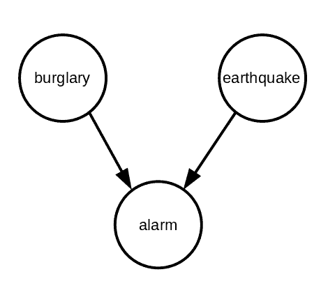
In Bayesian nets, the nodes are the events, and the edges represent dependence. In this example, alarm depends on burglary and earthquake, so there are arrows from these two events to the alarm. Using such a diagram and the definition for the joint probability of these events (next section), we can answer questions like the ones we mentioned above.
In this section, we formally define Bayesian networks and explain some of their characteristics, such as consistency of the sub-networks, the explaining away property, and the Markov blanket.
Bayesian networks are a type of probabilistic graphical models. Let’s say that we have events. We can represent them with random variables  ,
,  , …,
, …,  . Then, we define a Bayesian net as a Directed Acyclic Graph (DAG) with its nodes representing the events and its edges representing the dependencies between the events. Each event has a local conditional distribution, and the whole graph represents the joint distribution over all the variables. We define this joint distribution to be the product of all the local conditional distributions in the network:
![\[P(X_1, X_2, ..., X_n) = \prod_{i=1}^n p(x_i|x_{parents_i})\]](/wp-content/ql-cache/quicklatex.com-490c6bc2aa72a1107c3bf09d4523e92a_l3.svg "Rendered by QuickLaTeX.com")
An interesting property of the BNs is that the occurrence of all the parents of a node will guarantee the occurrence of the child. In mathematical terms:
![\[\sum_{X_i} p(X_i | X_{parents(i)}) = 1\ \textnormal{for each}\ X_{parents(i)}\]](/wp-content/ql-cache/quicklatex.com-4ccf303ccc261ca8fbf046d0f07f2253_l3.svg "Rendered by QuickLaTeX.com")
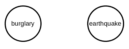
This leads the sub-networks of a BN to be consistent, meaning that they’re also Bayesian networks. We can show this by marginalizing on the alarm event in our example above and calculating the joint distribution of burglary and earthquake:
![\[p(b, e) = \sum_a p(b, e, a) = \sum_a p(b)p(e)p(a|b, e)\]](/wp-content/ql-cache/quicklatex.com-1aa97d88b57d0018ef283c35cdc18ee4_l3.svg "Rendered by QuickLaTeX.com")
since
![\[p(a|b, e) = 1,\]](/wp-content/ql-cache/quicklatex.com-d49b05253b90f166459074a0f3412d09_l3.svg "Rendered by QuickLaTeX.com")
we’ll have
![\[p(b, e) = p(b)p(e)\]](/wp-content/ql-cache/quicklatex.com-38a78228b67632f54126633664fbaffa_l3.svg "Rendered by QuickLaTeX.com")
which is the definition of a BN on the two events and graphical representation is:
In our example above, we have two causes (burglary and earthquake) for an event (alarm). Without knowing if there’s an alarm or not, the two causes are independent of each other, meaning that knowing one of them won’t influence the other one. However, if we know that the alarm has gone off, then knowing about one of the causes will reduce the probability of the other cause. This phenomenon is the explaining away the property of BNs.
For instance, let’s assume that we have the above-mentioned example with  . Therefore, we’ll have
  . Now, if we hear the alarm, what’s the probability of the burglary causing it? In other words, we want to calculate
  . According to the rules of conditional probability:
![\[p(b|a) = \frac{p(a\cap b)}{p(a)} = \frac{p(b)p(a|b)}{p(a)} = \frac{\epsilon \times 1}{p(a)}\]](/wp-content/ql-cache/quicklatex.com-918ed2d2e0d040599129efa5eb0d4889_l3.svg "Rendered by QuickLaTeX.com")
To calculate , we can consider the situations in which it’ll happen. The alarm will go off if either burglary happens and earthquake does not happen ( ), or vice versa (
 ), or both of them happen (
 ). As a result, we’ll have:
![\[p(a) = \epsilon (1-\epsilon) + \epsilon (1-\epsilon) + \epsilon^2 = \epsilon(2-\epsilon)\]](/wp-content/ql-cache/quicklatex.com-a63f626dba43ea10547f6c54799ae05c_l3.svg "Rendered by QuickLaTeX.com")
Consequently,
![\[p(b|a) = \frac{1}{2-\epsilon} = \frac{1}{1.95} \sim 0.51\]](/wp-content/ql-cache/quicklatex.com-ebbe414e48e6f4731e1669e4df5648ad_l3.svg "Rendered by QuickLaTeX.com")
However, if we know that earthquake has happened, we’ll have:
![\[p(b)\times p(\neg e) = 0\]](/wp-content/ql-cache/quicklatex.com-c76cd91b68dca0076be53d3d5d10a0d3_l3.svg "Rendered by QuickLaTeX.com")
![\[p(\neg b)\times p(e) = 1-\epsilon\]](/wp-content/ql-cache/quicklatex.com-b54b44388551fdb7becfe1184cca50fb_l3.svg "Rendered by QuickLaTeX.com")
![\[p(b)p(e) = \epsilon\]](/wp-content/ql-cache/quicklatex.com-6614ce1700063aff1936b73d242ca1de_l3.svg "Rendered by QuickLaTeX.com")
Therefore:
![\[p(a) = 1-\epsilon + \epsilon = 1\]](/wp-content/ql-cache/quicklatex.com-2713473691c494756dd8678ff4660875_l3.svg "Rendered by QuickLaTeX.com")
As a result:
![\[p(b|a, e) = \epsilon\]](/wp-content/ql-cache/quicklatex.com-a01ca35d4c97aebe4ba31ed314ff19dc_l3.svg "Rendered by QuickLaTeX.com")
This shows that knowing one of the causes reduces the probability of the other cause.
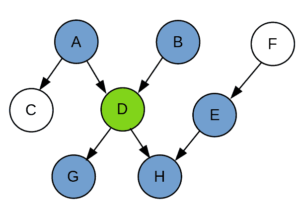
Given a node, Markov blanket is the set of its parents, children, and parents of its children. In other words, the Markov blanket separates the node from the rest of the network. Consequently, every node becomes independent of all other nodes given its Markov blanket. For example, in the graph below, the set of  is the Markov blanket of the node D:
The inference is asking questions (queries) about a model or network. To do that, there are several algorithms that we can use. Here, we explain three of these algorithms.
Hidden Markov Models (HMMs) are a special case of Bayesian networks that are suitable for modeling sequential events such as object tracking. In HMMs, we can have two types of states, namely hidden and observed. An arrow indicates a transition from one state to the next state with a transition probability. It can also connect a hidden state to an observed state with an emission probability. Given the observed states, we’d like to find out about the hidden states of HMMs:
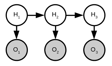
Probabilistic inference in HMMs can be finding an assignment for hidden states given the observed data. To do that, we can use the forward-backward algorithm, which uses dynamic programming to compute the weight of a path from the beginning to the end. Let’s keep in mind that the weight is the objective we’d like to optimize. In addition, we define it as the product of local weights  or probabilities similar to the definition of the joint distribution in BNs that we mentioned in Section 4. To calculate the path weight, we can use the lattice representation:
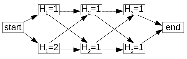
In the lattice above, we assume that there are three hidden states and each state can take on two values. Then, for every state, we can calculate a forward weight and a backward weight using the following formulas:
Forward weight:
![\[F_i(h_i) = \sum_{h_{i-1}} F_{i-1}(h_{i-1})w(h_{i-1}, h_i)\]](/wp-content/ql-cache/quicklatex.com-8f437aa2ebb5eb1e608deee864bc7403_l3.svg "Rendered by QuickLaTeX.com")
Backward weight:
![\[B_i(h_i) = \sum_{h_{i+1}} B_{i+1}(h_{i+1})w(h_i, h_{i+1})\]](/wp-content/ql-cache/quicklatex.com-d830f866997cd28dc3f4213a3dfb85a2_l3.svg "Rendered by QuickLaTeX.com")
In the end, the weight of a path form start to end that goes through the state  will be:
![\[S_i(h_i) = F_i(h_i) B_i(h_i)\]](/wp-content/ql-cache/quicklatex.com-4175669b16facb1f809a39926d1419bb_l3.svg "Rendered by QuickLaTeX.com")
The forward-backward algorithm was an exact algorithm to do probabilistic inference. However, this can be problematic as the number of values that each state can take on increases. As a result, we’ll have to resort to approximate algorithms.
Particle filtering is an approximate algorithm that is similar to beam search in that it has similar steps of extending and pruning. It also tries to solve some of the problems in beam search, such as its being slow and greedy.
Particle filtering consists of three steps: propose, weight, and resample. Let’s assume that we have our HMM example above, and we have already chosen two hidden states or particles  . Now, we want to select a value for one more particle
  . In the proposed step, we extend the existing particles based on the transition probability from the least particle to the new one.
The newly chosen candidate will have an observed state. Then, in the weight step, we calculate the weight of the three states  with different proposals that cause the new evidence. These are the weights that we’ll use in the resampling step to pruning the candidates. In the resampling step, based on the weights of each particle, we sample K times independently from that distribution. Let’s keep in mind that in the beam search, we would choose top K particles. However, in particle filtering, we sample from the distribution K times independently. Resampling gives a high probability to particles with large weights, but low weight particles also possibly appear in our draws.
Here’s the algorithm for particle filtering:

Gibbs sampling is another way to draw samples from a probability distribution. In Gibbs sampling, we initially assign random values to the hidden states (i.e., a random complete assignment). Then, going through all the variables one by one, we keep all the variables the same except the current variable. Then, for that variable, we choose a value that maximizes the product of the variables. We repeat this until convergence.
Here’s the algorithm for Gibbs sampling in a setting for probabilistic inference:
algorithm GibbsSampling(BayesianNet):
    // INPUT
    //    BayesianNet = the Bayesian network to sample from
    // OUTPUT
    //    An updated complete assignment

    x <- a random complete assignment

    for i <- 1 to n:
        for each v:
            Compute the weight of x + {X_i : v}
        Choose x + {X_i : v} with the probability proportional to weights

return xIn order to ask questions and do inference with BNs, we need to know the local conditional distributions. Therefore, we can say that these distributions are the parameters of our network, and we need to find a way to learn them. As a result, we should have or collect some training data to calculate the prior distributions. Then, we can think of some algorithms to learn the parameters from the data. In this section, we go over some of the algorithms.
We can learn the parameters of a BN by simply counting the number of times an event happens and then by normalizing the numbers. Here’s an algorithm that does so:
algorithm SupervisedLearning(D_train):
    // INPUT
    //    D_train = Training examples
    // OUTPUT
    //    θ = {p_d : d in D_train}

    // Count
    for x in D_train:
        for each x_i:
            Increment count_d(x_Parents(i), x_i)

    // Normalize
    for each d and local assignment x_Parents(i):
        p_d(x_i | x_Parents(i)) <- proportional to count_d(x_Parents(i), x_i)

    return p_d
The above algorithm corresponds to Maximum Likelihood for Bayesian networks since it maximizes the product of the variables.
Since our algorithm works based on the number of times an event occurs, it could run into trouble if we didn’t have some events in the training data. The probability of those would be set to zero, and the model would overfit. For instance, in a coin flip, by seeing heads five times after flipping the coin five times, the maximum likelihood will set the probability of tails to zero. Consequently, the prediction for the next flips would always be headed.
To solve this issue, we can give a prior count (lambda) to all the possible events in the network. That’ll make sure that their probability is never zero. The name of this method is Laplace smoothing, and the additional count can vary depending on the problem. However, we can usually set that to one.
In learning the parameters so far, we assumed that we had completed assignments of the variables. However, it often happens that some values are missing, and we only have partial assignments. In this case, first, we need to estimate the missing values. Then, we can learn from the now completed assignments.
With the Expectation-Maximization (EM) algorithm, we can find the missing values and learn the network parameters. The EM algorithm consists of two steps, E-step and M-step. In the E-step, we infer the hidden variables using one of the inference algorithms that we covered in the last section. After that, in the M-step, we use maximum likelihood estimation and Laplace smoothing, if necessary, to find the parameters.
The EM algorithm will result in a local optimum. However, to increase our chances of ending up in the global optimum, we can use random initialization.
In this article, we described in detail the Bayesian Networks (BNs). First, with a real-life example, we motivated the use of BNs. Then, we defined them mathematically and learned about how we can use these models in order to understand the hidden reasons behind an event that we might observe. Moreover, we went over the methods for parameter learning in BNs. Finally, we learned how to do inference using exact and approximate algorithms.