Gradient Descent Equation in Logistic Regression

1. Introduction

In this tutorial, we’re going to learn about the cost function in logistic regression, and how we can utilize gradient descent to compute the minimum cost.

2. Logistic Regression

We use logistic regression to solve classification problems where the outcome is a discrete variable. Usually, we use it to solve binary classification problems. As the name suggests, binary classification problems have two possible outputs.

We utilize the sigmoid function (or logistic function) to map input values from a wide range into a limited interval. Mathematically, the sigmoid function is:

$y = g(z) = \frac{1}{1 + e^{-z}} = \frac{e^z}{1 + e^z}$

This formula represents the probability of observing the output $y = 1$ of a Bernoulli random variable. This variable is either $1$ or $0$ ( $y \in {0,1}$ ).

It squeezes any real number to the $(0,1)$ open interval. Thus, it’s better suited for classification. Moreover, it’s less sensitive to outliers, unlike linear regression:

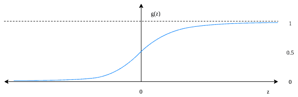
Applying the sigmoid function on $0$ gives $0.5$ . The output becomes $1$ as the input approaches $\inf$ . Conversely, sigmoid becomes $0$ as the input approaches $- \inf$ .

More formally, we define the logistic regression model for binary classification problems. We choose the hypothesis function to be the sigmoid function:

$h_{\theta}(x) = \frac{1}{1+e^{-\theta^T x}}$

Here, $\theta$ denotes the parameter vector. For a model containing $n$ features, we have $\theta = [\theta_0, \theta_1, ..., \theta_n]$ containing $n + 1$ parameters. The hypothesis function approximates the estimated probability of the actual output being equal to $1$ . In other words:

$P(y=1| \theta, x) = g(z) = \frac{1}{1+e^{-\theta^T x}}$

and

$P(y=0| \theta, x) = 1 - g(z) = 1 - \frac{1}{1+e^{-\theta^T x}} = \frac{1}{1 + e^{\theta^T x}}$

More compactly, this is equivalent to:

$P(y | \theta, x) = \left(\frac{1}{1 + e^{-\theta^T x}} \right)^y \times \left(1- \left(\frac{1}{1 + e^{\theta^T x}} \right) \right)^{1-y}$

3. Cost Function

The cost function summarizes how well the model is behaving. In other words, we use the cost function to measure how close the model’s predictions are to the actual outputs.

In linear regression, we use mean squared error (MSE) as the cost function. But in logistic regression, using the mean of the squared differences between actual and predicted outcomes as the cost function might give a wavy, non-convex solution; containing many local optima:

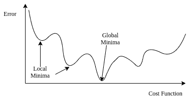
In this case, finding an optimal solution with the gradient descent method is not possible. Instead, we use a logarithmic function to represent the cost of logistic regression. It is guaranteed to be convex for all input values, containing only one minimum, allowing us to run the gradient descent algorithm.

When dealing with a binary classification problem, the logarithmic cost of error depends on the value of $y$ . We can define the cost for two cases separately:

$cost(h_{\theta}(x),y) = \left\{ \begin{array}{lr} - log(h_{\theta}(x)) & \text{, if } y = 1\\ - log(1-h_{\theta}(x)) & \text{, if } y = 0 \end{array}$

Which then results in:

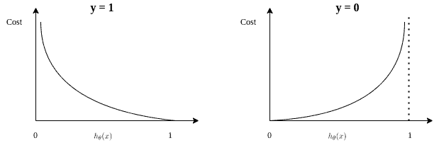
Because when the actual outcome $y = 1$ , the cost is $0$ for $h_{\theta}(x) = 1$ and takes the maximum value for $h_{\theta}(x) = 0$ . Similarly, if $y = 0$ , the cost is $0$ for $h_{\theta}(x) = 0$ .

As the output can either be ${0}$ or ${1}$ , we can simplify the equation to be:

$cost(h_{\theta}(x),y) = - y^{(i)} \times log(h_{\theta}(x^{(i)})) - (1-y^{(i)}) \times log(h_{\theta}(x^{(i)}))$

For $m$ observations, we can calculate the cost as:

$J(\theta) = - \frac{1}{m} \sum_{i=1}^{m} \left[ y^{(i)} \times log(h_{\theta}(x^{(i)})) + (1-y^{(i)}) \times log(h_{\theta}(x^{(i)})) \right]$

4. Minimizing the Cost with Gradient Descent

Gradient descent is an iterative optimization algorithm, which finds the minimum of a differentiable function. In this process, we try different values and update them to reach the optimal ones, minimizing the output.

In this article, we can apply this method to the cost function of logistic regression. This way, we can find an optimal solution minimizing the cost over model parameters:

$\min_\theta J(\theta)$

As already explained, we’re using the sigmoid function as the hypothesis function in logistic regression.

Assume we have a total of $n$ features. In this case, we have $n$ parameters for the $\theta$ vector. To minimize our cost function, we need to run the gradient descent on each parameter $\theta_j$ :

$\theta_j \gets \theta_j - \alpha \frac{\partial}{\partial \theta_j} J(\theta)$

Furthermore, we need to update each parameter simultaneously for each iteration. In other words, we need to loop through the parameters $\theta_0$ , $\theta_1$ , …, $\theta_n$ in vector $\theta = [\theta_0, \theta_1, ..., \theta_n]$ .

To complete the algorithm, we need the value of $\frac{\partial}{\partial \theta_j} J(\theta)$ , which is:

$\frac{\partial}{\partial \theta_j} J(\theta) = \frac{1}{m} \sum_{i=1}^{m} \left( h_{\theta}(x^{(i)}) - y^{(i)} \right) x_j^{(i)}$

Plugging this into the gradient descent function leads to the update rule:

$\theta_j \gets \theta_j - \alpha \frac{1}{m} \sum_{i=1}^{m} \left( h_{\theta}(x^{(i)}) - y^{(i)} \right) x_j^{(i)}$

Surprisingly, the update rule is the same as the one derived by using the sum of the squared errors in linear regression. As a result, we can use the same gradient descent formula for logistic regression as well.

By iterating over the training samples until convergence, we reach the optimal parameters $\theta$ leading to minimum cost.

5. Conclusion

In this article, we’ve learned about logistic regression, a fundamental method for classification. Moreover, we’ve investigated how we can utilize the gradient descent algorithm to calculate the optimal parameters.

Full Archive

About Baeldung

Core Concepts

Operating Systems

Artificial Intelligence

Graph Theory

Latex

1. Introduction

2. Logistic Regression

3. Cost Function

4. Minimizing the Cost with Gradient Descent

5. Conclusion