

Learn through the super-clean Baeldung Pro experience:
>> Membership and Baeldung Pro.
No ads, dark-mode and 6 months free of IntelliJ Idea Ultimate to start with.
Learn through the super-clean Baeldung Pro experience:
>> Membership and Baeldung Pro.
No ads, dark-mode and 6 months free of IntelliJ Idea Ultimate to start with.
In this tutorial, we’ll explore vertex coloring in graphs.
A graph  is a collection of nodes (vertices)
  and edges
  such that every edge
  joins two vertices from . For example:

We look at the problem of coloring all nodes of a loopless graph with unique colors. To clarify, a loopless graph is one in which no node has an edge connecting it to itself.
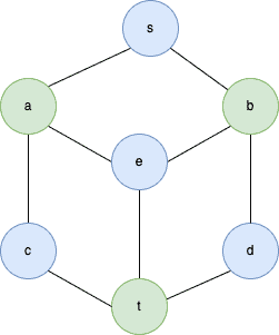
Vertex (or node) coloring of  means finding an assignment
  that colors each vertex so that no two neighboring vertices have the same color. For instance:
Formally, a proper vertex coloring  of
of  is a mapping
  , where
  are colors, such that no two adjacent vertices have the same color:
![\[(\forall u, v \in V) ((\exists e \in E)(e\text{ joins }u\text{ and }v)) \implies f(u) \neq f(v)\]](/wp-content/ql-cache/quicklatex.com-e29610ea79edc0a79fead684a83bcb6c_l3.svg "Rendered by QuickLaTeX.com")
If there’s a proper coloring of a graph with  colors, we say that is -colorable.
We define the chromatic number of (denoted by  ) as the minimum number of colors required to vertex color . In other words, it’s the smallest
  such that is -colorable.
First, for a graph where  , it holds that
  . Second, for a complete graph ,
  since each vertex is connected to the remaining
  vertices. On similar lines,
  where is a null graph.
Moving on, if  is a sub-graph of , then
  . This is intuitive since would need no more colors than because has no more nodes than .
Determining the chromatic number for a generic graph is an NP-complete problem.
These problems are of great interest to computer scientists because they arise in many practical applications, but no algorithm with the worst-case polynomial complexity is known to solve them.
The nodes of a -colorable graph can be partitioned into independent sets:  . Here, no two vertices in a set are adjacent to each other.
For our vertex-coloring example graph  , we have
  , so
, so  and
and  . Both
  and
and  are independent as
  and
and  .
.
In this section, we present a greedy algorithm for determining the chromatic number of a graph. It isn’t an exact algorithm, which means it returns an upper bound on  :
:
algorithm GraphColoring(G):
    // INPUT
    //    G = the graph to color with vertices V and edges E
    // OUTPUT
    //    K = the chromatic number
    //    Colors = the color assignment for each node

    // Initialize Colors to -1 to mark all vertices as unlabelled (white)
    Colors <- initialize an array with |V| elements
    for v in V:
        Colors[v] <- -1

    // Sort the vertices in descending order based on their degrees
    S_V <- Sort(V)

    // Assign the smallest available color to each vertex
    for v in S_V:
        AvailableColors <- {1, 2, ..., N}
        for u in neighbors(v):
            if Colors[u] in AvailableColors:
                AvailableColors <- AvailableColors \ {Colors[u]}
        Colors[v] <- MIN(AvailableColors)

    // Calculate the chromatic number K
    K <- MAX(Colors)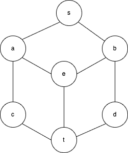
return K, ColorsWe start with the given graph  with .
Firstly, we set the colors of all the nodes -1 to denote that all vertices at the start are uncolored (white).
Then, we iterate over the nodes sorted by their degrees. There are  options for each node in the beginning (
 ). We disregard the colors assigned to its neighbors and give it the minimal color code remaining in .
After processing all the nodes, the algorithm returns the maximum color code as the chromatic number. Since this is a greedy algorithm, the returned number is only an estimate and should be treated as the upper bound of .
The time complexity of this algorithm depends on how we implement and  . If we use hash tables, the overall time complexity will be
  .
.
The space complexity is also  because of the upper bound on the number of edges in a graph with nodes.
Let’s check out an example:
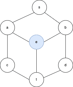
Initially, all the nodes are white (![(\forall v \in V) Colors[v] = -1](/wp-content/ql-cache/quicklatex.com-22d1dbad5240ebddaadd8f2f4d4ce693_l3.svg "Rendered by QuickLaTeX.com") ). Since there are seven nodes, each vertex in the main loop will start with seven available colors. Let their codes be
). Since there are seven nodes, each vertex in the main loop will start with seven available colors. Let their codes be  blue=1, green=2, red=3, pink=4, black=5, brown=6, violet=7
 .
.
We start with vertex  , which has the highest degree (3). Its neighbors are
  . All are white, so we color as blue since that’s the minimum of
  :
:
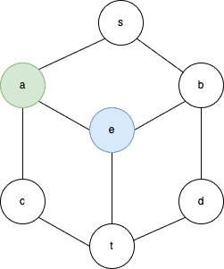
Next, we take vertex  . Its neighbors are
  . Since is blue, we disregard the color 1 and assign the minimum of the remaining codes (2):
Now comes the turn of  . Its neighbors are
  . The reasoning is the same as for , so we color it green:
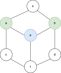
Continuing like this, we color this graph using two colors (blue and green), which gives us .
This enables us to run various operations on graphs to solve specific problems.
Here, we consider the problem of scheduling exams in a university. Typically, we have different subjects and will have many students enrolled in each subject. Further, each student can be enrolled in more than one subject, and each subject will have more than one enrolled student.
We need to schedule exams such that no two exams with at least one common student are on the same day. Additionally, we want to schedule all exams in the minimal possible number of days. How do we solve this? Vertex coloring comes to our rescue:
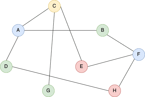
We represent this problem as a graph where we model each subject as a vertex. We introduce an edge between two vertices if the corresponding subjects have at least one student in common. Then, we find the graph’s chromatic number. It’s equal to the minimum number of days necessary to schedule all the exams simultaneously without a clash.
In our example, we’ll have 8 exams over 4 days.
Another application comes from the frequency assignment to radio towers. Here, we have several towers and need to use the smallest number of frequencies for communication.
Again, we model this as a graph coloring problem where we set each tower as a vertex. Then, we construct an edge between two towers if they are in interfering range with each other. After that, we apply vertex coloring and get our chromatic number, which shows us the minimal number of frequencies we need.
In this article, we studied vertex coloring in graphs and finding the chromatic number. An excellent way to understand this problem is to consider it an optimization problem. Given a graph , we minimize the number of colors needed to color it so that no two neighbors have the same color.
This problem has diverse applications, including clustering, data mining, digital image processing, computer networks, resource allocation, unconstraint optimization, and process scheduling.