Learn through the super-clean Baeldung Pro experience:
>> Membership and Baeldung Pro.
No ads, dark-mode and 6 months free of IntelliJ Idea Ultimate to start with.
Last updated: October 16, 2025

Learn through the super-clean Baeldung Pro experience:
>> Membership and Baeldung Pro.
No ads, dark-mode and 6 months free of IntelliJ Idea Ultimate to start with.
Fourier Analysis has taken the heed of most researchers in the last two centuries. One can argue that Fourier Transform shows up in more applications than Joseph Fourier would have imagined himself!
In this tutorial, we explain the internals of the Fourier Transform algorithm and its rapid computation using Fast Fourier Transform (FFT):
We discuss the intuition behind both and present two real-world use cases showing its importance.
Expanding a Function into a summation of simpler constituent Functions has redirected several scientists to tune into understanding numerous fields, e.g., overtones, wireless frequencies, harmonics, beats, and band filters. When Fourier first introduced his analysis and the possibility of expressing a periodic function (e.g.,  ) using a sum of periodic functions, he ran into multiple criticisms.
For example, Laplace (who was “the” physicist of his time) could not believe that a  series could express a
  . In 1811, Fourier resubmitted his work with an important addition, the Fourier Transform, which showed that not exclusively it is possible to expand Periodic Functions but non-Periodic ones too.
The study of Linear Systems and Signal Processing recognized the importance of Fourier Transforms. However, it did not reflect on numerical computation because of the number of arithmetic operations needed to calculate the discrete version of the Fourier Transform. At least that was the case until James Cooley and John Tukey introduced the Fast Fourier Transform algorithm.
The Discrete Fourier Transform of  points is given by:
![\[A_{i} = \sum_{j=0}^{n-1} \omega_{n}^{ij}a_j, \qquad i = 0, 1, . . ., n-1,\]](/wp-content/ql-cache/quicklatex.com-4f03942845a5331a2915246efcc11814_l3.svg "Rendered by QuickLaTeX.com")
Where
![\[\begin{split} \omega_n & = e^{2\pi i/n} \qquad\text{the } n^{th} \text{ root of 1; referred to as ``De Moivre's number" or the ``root of unity"} \\ & = cos^2(\frac{2\pi i}{n}) + sin^2(\frac{2\pi i}{n}) \end{split}\]](/wp-content/ql-cache/quicklatex.com-9032abe36fa766a7e7b1468a92f11629_l3.svg "Rendered by QuickLaTeX.com")
 and its powers construct the Fourier Transform. Although has two forms, using the exponential one (
 ) should serve us better in understanding its behavior.
Let  ;
;  will be the first root.
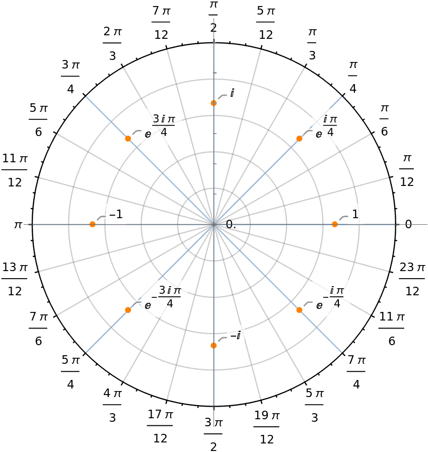
The figure below shows the eight different roots where is the first blue line, making a 45 degree ( ), and each of the following blue lines (also where the annotations are) will be the
  root of
  for
for  :
:
We can think of the multiplication between the different powers of and the input sequence as asking each  to capture the frequency it senses from the current input sequence. When the sum is infinite (i.e., having too many
  ‘s sensing the frequencies), it converges to the exact input sequence:
Each computation of  requires (complex) multiplication and
  (complex) additions. Hence, the complexity of total computation is
  (complex) multiplications and
  (complex) additions, complexity of
  .
.
The observation made by Cooley and Tukey was that if  is a composite number, a reduction in complexity exists. We can notice that as we square
  , we get
  .
.
For example,  is
is  .
.  for
for  :
:
To start our optimization attempt, it would be easier to work with and understand the vector notation of DFT:
![\[\underset{n\times 1}{\mathrm{A}} = \underset{n \times n}{F(n)} \times \underset{n\times 1}{a}\]](/wp-content/ql-cache/quicklatex.com-7ebfaa8e28262207d2c5ac50ddabb0cd_l3.svg "Rendered by QuickLaTeX.com")
Where
![\[F(n) = \begin{bmatrix} \omega^{00} & \omega^{01} & \dots & \omega^{0(n-1)} \\ \omega^{10} & \omega^{11} & \dots & w^{1(n-1)}\\ \vdots & \vdots & \ddots & \vdots \\ \omega^{(n-1)0} & w^{(n-1)1& \dots & \omega^{(n-1)^2} \end{bmatrix} = \begin{bmatrix} 1 & 1 & \dots & 1 \\ 1 & \omega^{11} & \dots & w^{1(n-1)}\\ \vdots & \vdots & \ddots & \vdots \\ 1 & w^{(n-1)1& \dots & \omega^{(n-1)^2} \end{bmatrix}\]](/wp-content/ql-cache/quicklatex.com-ef232365d8f76fca4983e4a17ed6a29a_l3.svg "Rendered by QuickLaTeX.com")
Now  is a mesmerizing matrix; we construct it, multiply it by a sequence, and get the Fourier Transform of that sequence. But, we want to multiply
  by
by  as quickly as possible.
Normally, such multiplication would take , and the optimization is possible if the matrix contained zeros, but the Fourier matrix has no zeros!
However, it is possible to make use of the special pattern  we previously learned so that can be factored in a way that produces many zeros (a.k.a FFT). The key idea is to connect to
  .
.
For instance, let  ; we would like to find the connection between
![\[F(4) = \begin{bmatrix} 1 & 1 & 1 & 1 \\ 1 & \omega & \omega^2 & \omega^3 \\ 1 & \omega^2 & \omega^4 & \omega^6 \\ 1 & \omega^3 & \omega^6 & \omega^9 \\ \end{bmatrix} = \begin{bmatrix} 1 & 1 & 1 & 1 \\ 1 & i & i^2 & i^3 \\ 1 & i^2 & i^4 & i^6 \\ 1 & i^3 & i^6 & i^9 \\ \end{bmatrix} \qquad \text{and} \qquad \begin{bmatrix} F(2) & \textbf{0} \\ \textbf{0} & F(2) \end{bmatrix} = \begin{bmatrix} 1 & 1 & 0 & 0 \\ 1 & i^2 & 0 & 0\\ 0 & 0 & 1 & 1 \\ 0 & 0 & 1 & i^2 \end{bmatrix}\]](/wp-content/ql-cache/quicklatex.com-dc76b839c9a12ec9d7b6db28126bb5f8_l3.svg "Rendered by QuickLaTeX.com")
So, we are somehow trying to reduce the number of operations by half, but these two matrices are not equal, yet. How about we add a permutation matrix that splits the input sequence into odd and even coordinates?
![\[\begin{bmatrix} F(2) & \textbf{0} \\ \textbf{0} & F(2) \end{bmatrix} \begin{bmatrix} \text{even-odd} \\ \text{permutation} \end{bmatrix} = \begin{bmatrix} 1 & 1 & 0 & 0 \\ 1 & i^2 & 0 & 0\\ 0 & 0 & 1 & 1 \\ 0 & 0 & 1 & i^2 \end{bmatrix} \begin{bmatrix} 1 & 0 & 0 & 0 \\ 0 & 0 &1& 0\\ 0 & 1 &0 & 0\\ 0 & 0& 0 & 1 \end{bmatrix} = \begin{bmatrix} 1 & 0 &1& 0 \\ 1 & 0 & i^2& 0 \\ 0 & 1 & 0 & 1\\ 0& 1 & 0& i^2 \\ \end{bmatrix}\]](/wp-content/ql-cache/quicklatex.com-78608cf533882e4657b0031e41de2f02_l3.svg "Rendered by QuickLaTeX.com")
At this point, we succeeded in producing a lot of zeros, but the factorized version seems far from being equal to the original  . However, we are pretty close, only if we can find a “fix-up matrix” to correct the previous output.
Let’s consider the following matrix:
![\[\begin{bmatrix} \text{fix up} \\ \text{matrix} \end{bmatrix} \begin{bmatrix} F(2) & \textbf{0} \\ \textbf{0} & F(2) \end{bmatrix} \begin{bmatrix} \text{even-odd} \\ \text{permutation} \end{bmatrix} = \begin{bmatrix} 1 & 0 & 1 & 0 \\ 0 & 1 & 0 & i\\ 1 & 0 & -1 & 0 \\ 0 & 1 & 0 & -i \end{bmatrix} \begin{bmatrix} 1 & 1 & 0 & 0 \\ 1 & i^2 & 0 & 0\\ 0 & 0 & 1 & 1 \\ 0 & 0 & 1 & i^2 \end{bmatrix} \begin{bmatrix} 1 & 0 & 0 & 0\\ 0&0 &1& 0\\ 0 & 1 & 0& 0 \\ 0&0&0 & 1 \end{bmatrix} = \begin{bmatrix} 1 & 1 & 1 & 1 \\ 1 & i & i^2 & i^3 \\ 1 & i^2 & i^4 & i^6 \\ 1 & i^3 & i^6 & i^9 \\ \end{bmatrix}\]](/wp-content/ql-cache/quicklatex.com-ad6d2d6bb30f38e1119458a61873fe24_l3.svg "Rendered by QuickLaTeX.com")
The new “fix up matrix” works on the reassembly of the half-sizes matrices. The form of that matrix is:
![\[\begin{bmatrix} I_n & D_n \\ I_n & -D_n \end{bmatrix} \qquad \text{and in our case is} \qquad \begin{bmatrix} I_4 & D_4 \\ I_4 & -D_4 \end{bmatrix}\]](/wp-content/ql-cache/quicklatex.com-f8a3eae4a7f48596f9f8d295bace4d17_l3.svg "Rendered by QuickLaTeX.com")
Where  is a diagonal matrix with entries
  and
and  is the identity matrix:
![\[D_n = \begin{bmatrix} 1 & 0 & 0 & \dots & 0 \\ 0 & \omega & 0 & \dots & 0 \\ 0 & 0 & \omega^2 & \dots & \vdots \\ \vdots & \vdots & \vdots & \ddots & 0 \\ 0 & 0 & \dots & 0 & \omega^{n-1} \end{bmatrix} \qquad \text{and} \qquad I_n = \begin{bmatrix} 1 & 0 & 0 & \dots & 0 \\ 0 & 1 & 0 & \dots & 0 \\ 0 & 0 & 1 & \dots & \vdots \\ \vdots & \vdots & \vdots & \ddots & 0 \\ 0 & 0 & \dots & 0 & 1 \end{bmatrix}\]](/wp-content/ql-cache/quicklatex.com-2d963e15308c8f8c2470ebc2252ca9b9_l3.svg "Rendered by QuickLaTeX.com")
The full form would be:
![\[F(n) = \begin{bmatrix} I_n & D_n \\ I_n & -D_n \end{bmatrix} \begin{bmatrix} F(n/2) & \textbf{0} \\ \textbf{0} & F(n/2) \end{bmatrix} \begin{bmatrix} \text{even-odd} \\ \text{permutation} \end{bmatrix}\]](/wp-content/ql-cache/quicklatex.com-93a2a41c0ce486edf400c01aae357618_l3.svg "Rendered by QuickLaTeX.com")
What comes next? We reduced to . Keep going to  , …,
, …,  . That’s recursion! There are
  levels, going from
  down to
  . Each level has
  multiplications from the diagonal
  ‘s, to reassemble the half-size outputs from the lower levels. This yields the final count
  ., which is
  .
.
Note: In case is not a power of  , we can pad the input sequence with
  ‘s.
‘s.
For  , it would take
  multiplications, where FFT would perform
  multiplications only.
Fourier Transform has an indispensable number of applications to be listed. We’ll cast a shadow on Acoustics and Convolution Theorem.
How can Shazam recognize a song/music in a matter of seconds? More surprisingly, it does so regardless it is listening to an intro, verse, or chorus:
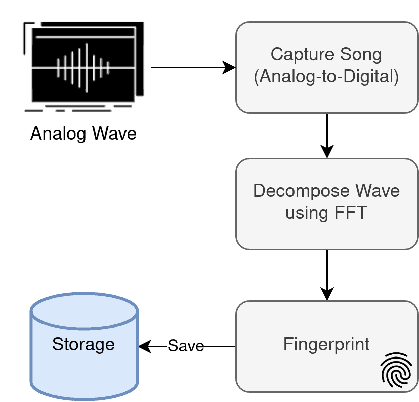
There are (roughly) four steps it performs:
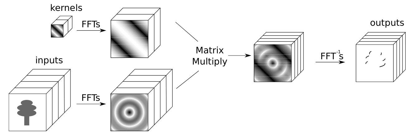
The theorem states that circular convolutions (i.e., periodic convolutions between two periodic functions having the same period) in the spatial domain are equivalent to point-wise products in the Fourier domain.
Let  denote the Fourier Transform and
  its inverse, we can compute convolutions between functions
  and
and  as follows
![\[f * g = \mathcal{F}^{-1}\{\mathcal{F}\{f\} \cdot \mathcal{F}\{g\}\}\]](/wp-content/ql-cache/quicklatex.com-5341181e5857479396932e0841c91095_l3.svg "Rendered by QuickLaTeX.com")
Originally, the convolution between and is calculated with
![\[f * g = \int_{-\infty}^{\infty} f(\tau) g(t - \tau) d\tau\]](/wp-content/ql-cache/quicklatex.com-9fc0dc4264d3b266ed5e172e862e580e_l3.svg "Rendered by QuickLaTeX.com")
A convolution of size  with a kernel size
  requires
  operations using the direct method, the complexity would be
  . On the other hand, FFT-based method would need
  operations with complexity
  :
:
The convolution operation is used in a wide variety of applications such as:
In this tutorial, we have provided a short mathematical analysis of the Fast Fourier Transform algorithm and how it can, surprisingly, impact a lot of fields and applications. The breakthrough of the algorithm only started a few decades ago even though Joseph Fourier introduced his analysis almost two centuries back.