What Is “Energy” in Image Processing? | Baeldung on Computer Science

1. Introduction

In this tutorial, we take a look at the term energy, as used in image processing. There are three different concepts of energy, in image processing, signal processing, and physics. All of them are closely related and we are going to focus on the part of image processing, shortly explaining the other two at the end of the article

2. Definition

The term energy describes the local change of a certain quality of the image. An example of quality would be brightness or intensity. Energy is specifically important for applications such as image compression. The reason for this lies in the fact that areas with a lot of energy contain a lot of information.

Furthermore, every grayscale image with $m \times n$ pixels can be described as an $m \times n$ matrix. The matrix entries represent the intensity, 0 being black and 255 being white. To understand the concept of local change better, let’s have a look at an example picture:

We can, for example, see a large local change between the face and the hair, as the face is very light and the hair is very dark:

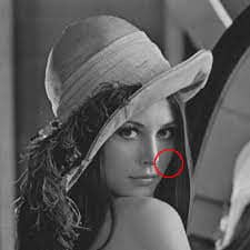
In image processing, this change in intensity is called an edge. The next question that arises is, how can we detect those changes automatically?

3. Fourier Transformations

To understand the Fourier transformation for images, we have to look at them as a 2-dimensional signal.

3.1. 1-Dimensional Fourier Transformation

Since a 2-dimensional signal might be a little bit overwhelming, we first look at a part of one row of our picture:

As we can see, the red pixels mark the circle we used in our example image. Removing them yields:

We already know that there is an edge there, now we only need to detect it with an algorithm. To do that we need a mathematical representation but how does this stripe look if we represent it mathematically, as an array of numbers?

$174 \ 188 \ 156 \ 108 \ 105 \ 104 \ 105 \ 102 \ 96 \ 87 \ 90 \ 73 \ 53 \ 29 \ 22 \ 30 \ 37 \ 39 \ 32 \ 44 \ 43 \ 42 \ 40$

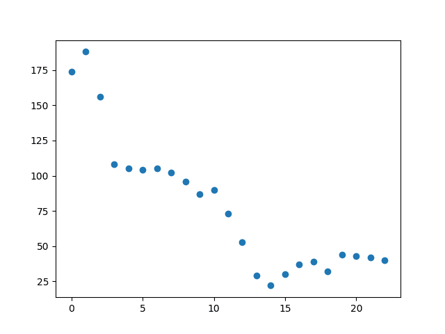
Let’s look at this array as a function, mapping each index to its corresponding entry. Then we can use the Fourier transform to retrieve the frequency spectrum of this function. As we can see our function is discrete, thus we are using the discrete Fourier transform. The frequency spectrum tells us exactly if we have an edge in our image and where it is.

Let’s visualize the spectrum:

We can see on the right, that we have a high frequency with a high magnitude as seen in yellow. This indicates a rough edge. If we want to detect edges, i.e. areas with high energy, we can simply filter out low frequencies.

3.2. Fourier Transformation for Images

After having a look at the concept of the Fourier transform in 1 dimension, let’s see how it works for our original image in 2 dimensions:

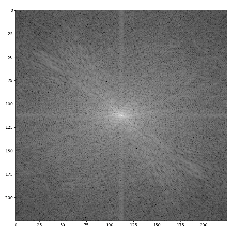
How can we interpret this image? Again, we see the frequency spectrum of our original image, but this time it is, as our original image, 2-dimensional. In the middle of our picture, we see the low frequency. The further we go outside of the centrum the higher frequency. To only display our edges, we simply reverse our Fourier transform, but only after removing the low frequencies in the center of our image:

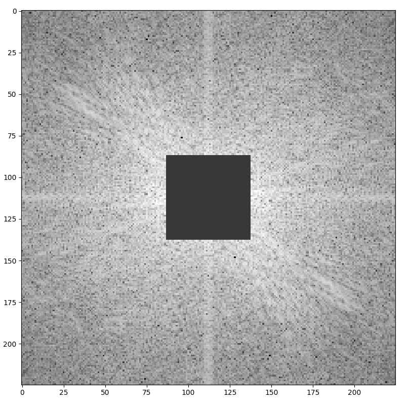
Frequency-domain-of-the-image-high-pass-filter

The inversed picture then looks like this:

4. Convolutions

Another way to detect edges, also including colored images, uses the method of convolution. It uses i.e. a $3 \times 3$ matrix that moves over our image, creating a weighted average of the pixels in a $3 \times 3$ area each step:

$g(x,y)=\omega * f(x,y) =\sum _{ w=-a }^{ a }{ \sum _{ z=-b }^{b}{ \omega ( w , z ) f ( x-w , y-z )}}$

$f$ describes our original image, mapping the intensity to each pixel

$g$ describes our filtered image

$\omega$ is our convolution matrix, also called filter kernel

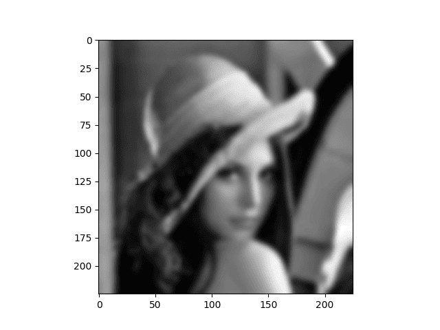
Doing so makes the image, as expected, blurrier:

We can then obtain the image of edges by subtracting the blurred image from our original one:

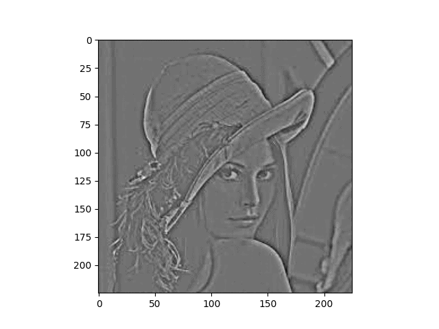
The convolution mask we used in this example is a gaussian kernel.

The formal definition of the energy of a function $x$ , in the sense of signal processing, is just the integral over the squared function:

$E_{s}\ \ =\ \ \langle x(t),x(t)\rangle \ \ =\int _{-\infty }^{\infty }{|x(t)|^{2}}dt$

In the discrete case we have:

$E_{s} \ \ =\ \ \langle x(n) , x(n)\rangle \ \ = \sum _{ n = -\infty }^{ \infty }{ |x(n)|^{2} }$

Applying the discrete case to image processing, we would simply add up the intensity of all our pixels. Thus, a completely white image would have the maximum energy and a black one zero, rendering this definition useless.

Meanwhile, the definition of energy we know from physics is closely related to the one from signal processing:

$E={E_{s} \over Z}={1 \over Z}\int _{-\infty }^{\infty }{|x(t)|^{2}}dt$

Here we only divide by the factor $\frac{1}{Z}$ , the magnitude of the signal.

6. Conclusion

In this article, we discussed the significance of energy in the area of image processing. We concluded that energy describes areas which contain lots of change. Additionally, we discussed how this energy can be detected automatically.

Full Archive

About Baeldung

Core Concepts

Operating Systems

Artificial Intelligence

Graph Theory

Latex