How to Prove That a Problem Is NP-Complete? | Baeldung on Computer Science

1. Introduction

There is still no proof of the problem whether $\mathcal{P} = \mathcal{NP}$ . The answer is likely to be “No”.

In this tutorial, assuming that $\mathcal{P} \neq \mathcal{NP}$ , we’ll learn how to prove the $\mathcal{NP}$ -Completeness of the problem. Also, we’ll take real algorithmic problems and prove that they are $\mathcal{NP}$ -Complete.

Finally, we’ll also use Big-O notation to describe time complexity.

2. NP-Hard and NP-Complete Problems

Let’s classify the decision problems – problems that have the “Yes” or “No” answers.

2.1. P and NP

The problem belongs to class $\mathbf{P}$ if it can be solved in polynomial time.

Similarly, the problem belongs to class $\mathbf{NP}$ if it can be solved in non-deterministic polynomial time. Intuitively, this set of problems is considered to be “hard” problems. Technically, we can’t solve them in polynomial time. However, their “runtime” might be a polynomial.

2.2. Reduction

Reduction of a problem $\mathbf{X}$ to problem $\mathbf{Y}$ $\mathbf{(X \leqslant_{p} Y)}$ is a conversion of inputs of problem $\mathbf{X}$ to the inputs of problem $\mathbf{Y}$ . This conversion is a polynomial-time algorithm itself. The complexity depends on the length of the input.

Let’s classify the inputs of the decision problems. “Yes” – input of the problem is the one that has a “Yes” answer to it. Likewise, “No” – input to the problem is the one that has a “No” answer to it.

If $\mathcal{X} \leqslant_{p} \mathcal{Y}$ then every “Yes” – input of $\mathcal{X}$ converts to “Yes” – input of $\mathcal{Y}$ . And every “No” – input of $\mathcal{X}$ converts to “No” – input of $\mathcal{Y}$ with the reduction algorithm. However, the alternate is that we can also prove that every “Yes” – input of $\mathcal{Y}$ converts to “Yes” – input of $\mathcal{X}$ , instead of working with no inputs. We’ll implement our own reduction algorithms later in the article.

Important to know, the polynomial reduction is a transitive relation. It means, that if problem $\mathcal{A}$ reduces to $\mathcal{B}$ with an algorithm $\alpha$ , and problem $\mathcal{B}$ reduces to $\mathcal{C}$ with an algorithm $\beta$ , then problem $\mathcal{A}$ reduces to $\mathcal{C}$ with an algorithm $\alpha \circ \beta$ . It can be achieved by applying algorithm $\alpha$ first to the inputs to the problem $\mathcal{A}$ . Then we’d get the inputs to the problem $\mathcal{B}$ and can apply algorithm $\beta$ to convert those inputs to the input to problem $\mathcal{C}$ .

2.3. NP-Hardness

The problem is $\mathbf{NP}$ -Hard if every problem from $\mathbf{NP}$ polynomially reduces to it. We may assume that $\mathcal{NP}$ -Hard problems are at least as hard as any problem in $\mathcal{NP}$ and might be even harder. However, the $\mathcal{NP}$ -Hard problem might or might not belong to $\mathcal{NP}$ .

2.4. NP-Completeness

The problem is $\mathbf{NP}$ -Complete if it belongs to $\mathbf{NP}$ , and every problem from $\mathbf{NP}$ polynomially reduces to it.

As we may notice, every $\mathcal{NP}$ -Complete problem is $\mathcal{NP}$ -Hard. But not every $\mathcal{NP}$ -Hard problem is $\mathcal{NP}$ -Complete. The example of $\mathcal{NP}$ -Hard but not the $\mathcal{NP}$ -Complete problem is the Halting Problem. This problem is hard but doesn’t belong to $\mathcal{NP}$ . Boolean satisfiability (SAT) is the first problem from $\mathcal{NP}$ that was proven to be $\mathcal{NP}$ -Complete. We can also find the 3SAT problem definition while reading about the Cook-Levin theorem.

3. Algorithm to Prove That a Problem Is NP-Complete

$\mathcal{NP}$ -Complete problems are the ones that are both in $\mathcal{NP}$ and $\mathcal{NP}$ -Hard.

So, to prove that problem is $\mathcal{NP}$ -Complete we need to show that the problem:

belongs to $\mathcal{NP}$
is $\mathcal{NP}$ -Hard

3.1. How to Show a Problem Is NP?

There exists a certificate verification strategy to show that the problem belongs to $\mathcal{NP}$ . A certificate is an answer to our problem. Verifier is a polynomial algorithm that can tell us whether the answer to the problem is “Yes” or “No”.

For instance, let’s take the Hamiltonian Cycle problem. The certificate to the problem might be vertices in order of Hamiltonian cycle traversal. We can check if this cycle is Hamiltonian in linear time. It is called verification. So, the problem belongs to $\mathcal{NP}$ . Moreover, it can be proven that the Hamiltonian Cycle is $\mathcal{NP}$ -Complete by reducing this problem to 3SAT.

3.2. How to Show a Problem Is NP-Hard?

To show that the problem is $\mathcal{NP}$ -Hard, we have to choose another $\mathcal{NP}$ -Hard problem and reduce the chosen problem to ours. Importantly, every $\mathcal{NP}$ -Hard problem is $\mathcal{NP}$ -Complete. Thus, we can also reduce any $\mathcal{NP}$ -Complete problem.

Remember, the relation of polynomial reduction is transitive. Therefore, we can reduce just one problem, not all the problems with $\mathcal{NP}$ .

3.3. Proof Strategy

Here are the main goals we need to achieve in order to prove the problem is $\mathcal{NP}$ -Complete:

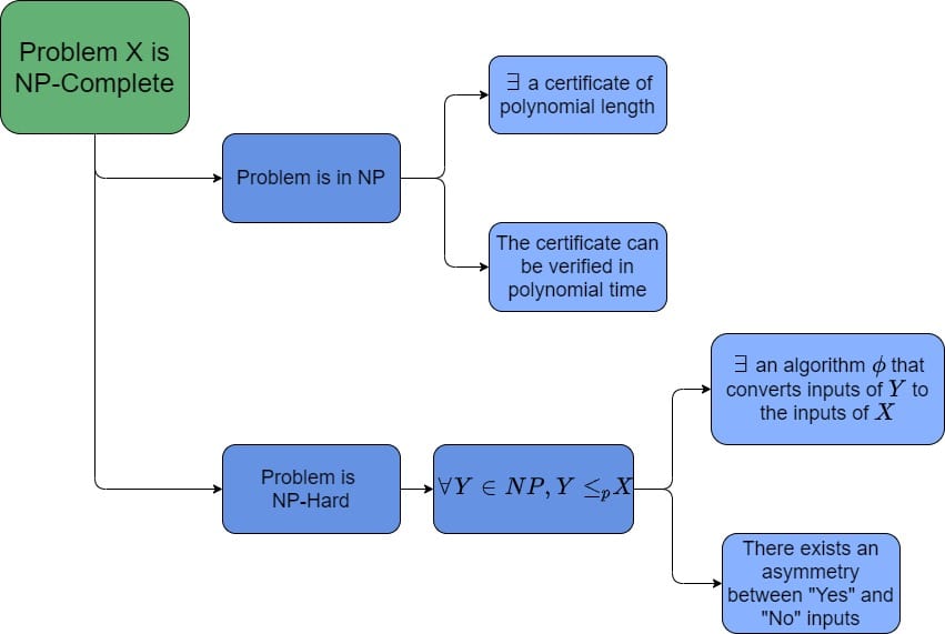
As mentioned, firstly, we have to prove that the problem is in $\mathcal{NP}$ class. If we cannot prove that, then we cannot move further. The $\mathcal{NP}$ -Complete problems always belong to $\mathcal{NP}$ .

When we choose a certificate, it must have a polynomial length. So, if the input to our problem is $n$ , but the length of the certificate is $O(2^n)$ , then we can’t verify this certificate. A verifier algorithm must have polynomial time complexity based on the length of the certificate.

After we checked that our problem is in $\mathcal{NP}$ , we have to prove that the problem is $\mathcal{NP}$ -Hard. The $\mathcal{NP}$ -Complete class of problems is the intersection of $\mathcal{NP}$ and $\mathcal{NP}$ -Hard. For any $\mathcal{NP}$ -Hard problem, we know that every problem from $\mathcal{NP}$ polynomially reduces to it.

We should also remember, that the reduction algorithm must convert “Yes” – and “No” – inputs of chosen $\mathcal{NP}$ -Hard or $\mathcal{NP}$ -Complete problem to the equivalent “Yes” – and “No” – inputs of our problem.

Let’s see two examples of proving that the problem is $\mathcal{NP}$ -Complete. We’ll reduce 3SAT to 4SAT and Independent Set problems.

4. 3SAT to 4SAT Reduction

Here is the 4SAT problem definition:

“Given a Boolean formula, which consists of $\mathbf{k}$ clauses, each clause is a disjunction of 4 literals or their negations. Is there an interpretation of variables such that every clause is satisfied?”

4.1. Certificate Verification of 4SAT

Firstly, let’s prove the problem belongs to $\mathcal{NP}$ . Suppose the formula has $n$ input variables. It means that the answer and our certificate is an interpretation of $n$ variables. They might be set to true or false. Moreover, we can check whether the formula is satisfied at a linear time. As a result, we verify our certificate in polynomial time. So, the problem is in $\mathcal{NP}$ .

4.2. Reduction of 3SAT to 4SAT

Secondly, we have to prove 4SAT is $\mathcal{NP}$ -Hard. Let’s take 3SAT, which is $\mathcal{NP}$ -Complete, and reduce 3SAT to 4SAT.

Our reduction gadget will be an algorithm, which converts inputs of 3SAT to the inputs of 4SAT.

Given an input 3SAT formula $\mathcal{A}$ , we construct the input formula $\mathcal{B}$ of 4SAT by expanding each clause with the new variable: $\mathcal{A}_{i} = (x \vee y \vee z) \implies (\x \vee y \vee z \vee h) \wedge (x \vee y \vee z \vee \neg h) = \mathcal{B}_{i}$ .

It is clear that we can do it in polynomial time. Let’s now check that “Yes” – inputs of 3SAT are converted to “Yes” – inputs of 4SAT and vice versa.

If a given clause $(x \vee y \vee z)$ is satisfied, then $(x \vee y \vee z \vee h) \wedge (x \vee y \vee z \vee \neg h)$ is satisfied. Variable $h$ can be either true or false. Thus, if $\mathcal{A}$ is satisfiable, $\mathcal{B}$ is satisfiable.

Suppose $\mathcal{B}$ is satisfied. Let the satisfiable interpretation of $n$ variables be $\mathcal{S}$ . $\mathcal{S}$ consists of assignments of each variable. Then $(x \vee y \vee z \vee h) \wedge (x \vee y \vee z \vee \neg h)$ must be true under $\mathcal{S}$ . Variables $h$ and $\neg h}$ have different values. If variable $h$ is true then $\neg h$ is false and vice versa. So, $(x \vee y \vee z)$ must be true under $\mathcal{S}$ as well. Thus, $\mathcal{A}$ is satisfiable.

As a result, we created a polynomial algorithm that converts the inputs of 3SAT to the inputs of 4SAT. It means that 4SAT is $\mathcal{NP}$ -Hard.

Finally, we’ve proved 4SAT is in $\mathcal{NP}$ and $\mathcal{NP}$ -Hard. Therefore, we can say that 4SAT is $\mathcal{NP}$ -Complete.

5. 3SAT to Independent Set Reduction

In graph theory, the Independent Set is a problem of finding a set of vertices of size $\mathbf{k}$ in a graph, such that no two of which are adjacent.

5.1. Certificate Verification of Independent Set

Let’s prove this problem belongs to $\mathcal{NP}$ . The certificate of the problem might be a set of chosen vertices. We can check in polynomial time whether any two of them are adjacent or no. Therefore, the problem is in $\mathcal{NP}$ .

5.2. Reduction of 3SAT to Independent Set

Suppose we have a 3SAT input formula, consisting of $k = 3$ clauses: $(x_{1} \vee \neg x_{3} \vee \neg x_{4}) \wedge (\neg x_{2} \vee x_{3} \vee x_{4}) \wedge (\neg x_{1} \vee x_{2} \vee x_{3})$ .

Let’s now reduce the 3SAT to Independent Set by building a graph, which would have an independent set of size $\mathbf{k}$ if and only if the given formula is satisfied. To do it, for each clause, we create a triangle graph and add the edges to all pairs of vertices, which consist of the variable and its negation:

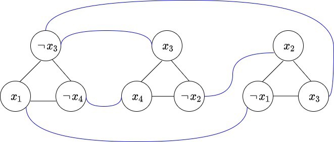
If a given formula is satisfied, then at least one variable in each clause is true. Let $\mathcal{S}$ be a set of such true variables. The formula consists of $k$ clauses. Thus, $k$ is the size of $\mathcal{S}$ , and the set of corresponding vertices in a built graph is independent and has a size of $k$ .

Next, if the graph has an independent set $\mathcal{S}$ of size $k$ , we know that it has one node from each “clause triangle.” We can set chosen variables to true. This is possible because no two are negations of each other, and the boolean formula will be satisfied.

We’ve proved already that the Independent Set problem is in $\mathcal{NP}$ and $\mathcal{NP}$ -Hard. Therefore, we can say that the Independent Set is $\mathcal{NP}$ -Complete.

6. Conclusion

In this tutorial, we’ve learned the most important definitions of the theory of complexities. Also, we’ve learned how to prove the $\mathcal{NP}$ -Completeness of the problem, using certificate verification and reduction strategy. Furthermore, we’ve shown two examples of $\mathcal{NP}$ -Completeness proof.

Full Archive

About Baeldung

Core Concepts

Operating Systems

Artificial Intelligence

Graph Theory

Latex