

Yes, we're now running our only Summer Sale. All Courses are 30% off until 20th July, 2026:
Learn through the super-clean Baeldung Pro experience:
>> Membership and Baeldung Pro.
No ads, dark-mode and 6 months free of IntelliJ Idea Ultimate to start with.
1. Introduction
We often need to be able to match two different sets of data together, such that as many elements as possible from one set are associated with an element from the other set.
For example, imagine scheduling appointments into available slots. If a professor has a fixed number of time slots available for consultations, and a number of students who want to take advantage of them, then we need to work out the most efficient way to match these together.
2. Maximum Bipartite Matching
A bipartite graph is a special case in graph theory because every vertex is in one of two distinct sets, often called  and
and  , and every edge connects between and . We can consider our two sets of data that we’re matching up to be the two sets and . The edges between the two are then the allowed connections.
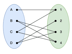
For example, in our case of a professor’s time slots and students, the vertices in could be the individual students, the vertices in could be the available slots, and the edges indicate which time slots each student is able to use:
A matching in graph theory, also known as an independent edge set, is a combination of edges where no two edges share the same vertex. This will often be a subset of all possible edges to then meet this requirement. The “maximum matching” is a matching that has the most number of edges possible. A “perfect matching” is one that uses every vertex in the graph, and therefore is the largest possible matching that we can achieve.
As such, the maximum matching of a bipartite graph is the maximum number of possible links between the two distinct sets, so that every link is between a different set of vertices. This can be a very useful concept since this is effectively the maximum number of pairings between two related sets; like between students and appointment slots for example.
3. Hopcroft-Karp Algorithm
The Hopcroft-Karp algorithm is an algorithm to generate a maximum matching for a given bipartite graph. This was developed by John Hopcroft and Richard Karp in 1973.
The algorithm works in phases, where each phase is looking for augmenting paths of increasing lengths. An augmenting path is any path starting and ending on unmatched vertices, where edges within the path alternate between unmatched and matched. We will always have an odd number of edges in these paths, but they could be of size 1 or up.
Each path we find is then used to increase the matching that we have so far. We do this by adding all previously unmatched edges into our matching, whilst removing all previously matched edges from the matching. This will have the effect of increasing the size of the matching by 1 for every path found.
For example, if we started from the following:
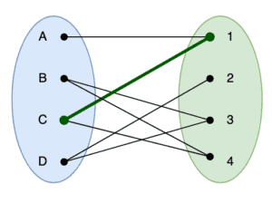
Here we have a single path between vertices  and
and  . We can find a new path that travels from
  , and add this to our matching. Doing so will end up with the following:
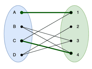
Here we can see that  gets removed from the matching, whilst adding
  and
and  into it. The end result is that we now have 2 paths in the matching.
4. Algorithm
The algorithm works in phases, where we perform a number of searches across the graph in each phase. We also do everything from the point of view of the vertices in , which helps simplify the number of steps required.
As input, the only thing that we require is the graph itself. Specifically, the details of which vertices in connect to which vertices in . Throughout the entire algorithm, we will also keep track of the matching. Specifically, which vertices in are currently paired with vertices in , though we need to be able to access this from both sides.
For each phase, we will additionally be keeping track of the current paths we have discovered. This is recorded as distances along the path for each vertex in . We don’t need to record distances for vertices in because these are only ever considered from the point of view of how they connect to vertices in .
4.1. Overall Algorithm
The overall algorithm starts with some general set up and then performs a number of searches grouped together in phases. During each phase, we perform a breadth-first search of the entire graph to discover any augmenting paths that exist in the graph. We then perform a number of depth-first searches, starting from each vertex in that is currently unmatched to build the appropriate augmenting paths and update the matching.
We also have a special vertex that is not part of the graph but is used in the algorithm. This is referred to as NIL, and we use this to indicate that a vertex in the graph is not currently paired with anything:
algorithm HopcroftKarp(U, V, Edges):
    // INPUT
    //    U = Set of vertices on one side of the bipartite graph
    //    V = Set of vertices on the other side of the bipartite graph
    //    Edges = List of edges connecting vertices in U to V
    // OUTPUT
    //    pairU = Matching of vertices in U to vertices in V
    pairU <- an empty int array of size U.length + 1
    pairV <- an empty int array of size V.length + 1
    for u in U:
        pairU[u] <- NIL
    for v in V:
        pairV[v] <- NIL
    pairU[NIL] <- NIL
    pairV[NIL] <- NIL
    running <- true
    repeat until not running:
        dist <- BFS(U, V, Edges, pairU, pairV)
        running <- (dist[NIL] != INF)
        if running:
            for u in U:
                if pairU[u] = NIL:
                    DFS(u, Edges, pairU, pairV, dist)
At the start of each phase, we perform a breadth-first search across the entire graph to discover if any augmenting paths exist, and the lengths of them. If we did not calculate a distance to the special NIL vertex, which indicates that we didn’t find any paths, then we will stop immediately. This means we have already reached the best matching possible.
If we did find an augmenting path, then we will expand our matching. This is done by iterating over every vertex in that is not currently paired and running a depth-first search across the graph starting from there. As part of this, we will be updating the matching, and swapping edges in and out as appropriate.
4.2. Breadth-First Search
The first part of each phase is the breadth-first search. We iterate over every vertex in and expand out to discover all of the augmenting paths that we can:
algorithm BFS(U, V, Edges, pairU, pairV):
    // INPUT
    //    U = Set of vertices on one side of the bipartite graph
    //    V = Set of vertices on the other side of the bipartite graph
    //    Edges = List of edges connecting vertices in U to V
    //    pairU <- an empty int array of size U.length + 1
    //    pairV <- an empty int array of size V.length + 1
    // OUTPUT
    //    dist = Distances along the path for each vertex in U
    workingQueue <- new Queue()
    for u in U:
        if pairU[u] = NIL:
            dist[u] <- 0
            workingQueue.push(u)
        else:
            dist[u] <- INF
    dist[NIL] <- INF
    while not workingQueue.empty():
        u <- workingQueue.pop()
        if dist[u] < dist[NIL]:
            for v in Edges[u]:
                paired <- pairV[v]
                if dist[paired] = INF:
                    dist[paired] <- dist[u] + 1
                    workingQueue.push(paired)
    return dist
We first discover every vertex in that is not currently part of the matching and add them to a working queue. We then iterate over this queue, looking at each vertex in turn.
For each of these, we iterate over every attached vertex in from the graph. We find the vertex from that is currently paired to this, which may be our special NIL vertex. If we’ve not yet calculated a distance for this, then we do so and add it to the working queue.
This then repeats until we run out of vertices to examine. At this point, we know every possible augmenting path through the graph from our current state, and we’re ready for the next step.
4.3. Depth-First Search
Once we’ve generated the current set of augmenting paths, we will start to expand them. We do this by performing a depth first search through the graph, from each vertex in that is not currently part of the matching. As we do this, we update the matching accordingly:
that is not currently part of the matching. As we do this, we update the matching accordingly:algorithm DFS(u, Edges, pairU, pairV, dist):
// INPUT
// u = Starting vertex in U
// U = Set of vertices on one side of the bipartite graph
// V = Set of vertices on the other side of the bipartite graph
// Edges = List of edges connecting vertices in U to V
// pairU <- an empty int array of size U.length + 1
// pairV <- an empty int array of size V.length + 1
// dist = Distances along the path for each vertex in U
// OUTPUT
// true if a matching can be expanded, false otherwise
if u != NIL:
for v in Edges[u]:
paired <- pairV[v]
if dist[paired] = dist[u] + 1:
if DFS(paired, Edges, pairU, pairV, dist):
pairV[v] <- u
pairU[u] <- v
return true
dist[u] <- INF
return false
return true5. Working Example
This is complicated, so the best way to follow it is to actually work along. Here we are using a very simple graph to make the demonstration shorter, but it will expand out to graphs of any size:
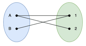
Our graph has two vertices on each side, and three edges between them. For example, it could represent a professor with morning and afternoon appointments available, and two students wishing to make use of them.
5.1. Phase 1
When we do the very first breadth-first search, this will discover a single augmenting path through the graph. This is between vertices  and . We don’t find any paths using vertices
  or
or  , because the only possible paths are using vertices that have already been used.
After this, we then perform depth-first searches starting from both and . The search starting from will add the edge into the matching, and the search starting from will add nothing:
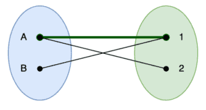
5.2. Phase 2
Our second breadth-first search will be starting from the above graph instead. In this case, we don’t need to investigate any paths from because it’s already in the matching, and so we instead start from . This will now discover the augmenting path that travels from  .
.
After this, we again perform the depth-first searches. As before, we only do this from since is already in the matching, and this will then add  and into the matching, whilst at the same time removing from the matching:
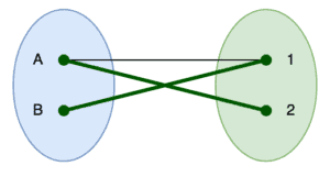
5.3. Phase 3
Our third breadth-first search has no vertices to start from because both and are already included. This means that we stop processing and return the matching that we have discovered so far. We can already see from looking at the above that this is the optimal matching.
6. Summary
In this article, we learned how we can match up two sets of data such that the most effective matching between them can be discovered. We’ve demonstrated it working on a small scale, but it will work equally effectively on much larger graphs as well.