Dijkstra Shortest Path Algorithm in Java
Last updated: May 11, 2024


Mocking is an essential part of unit testing, and the Mockito library makes it easy to write clean and intuitive unit tests for your Java code.
Get started with mocking and improve your application tests using our Mockito guide:
Handling concurrency in an application can be a tricky process with many potential pitfalls. A solid grasp of the fundamentals will go a long way to help minimize these issues.
Get started with understanding multi-threaded applications with our Java Concurrency guide:
Spring 5 added support for reactive programming with the Spring WebFlux module, which has been improved upon ever since. Get started with the Reactor project basics and reactive programming in Spring Boot:
Since its introduction in Java 8, the Stream API has become a staple of Java development. The basic operations like iterating, filtering, mapping sequences of elements are deceptively simple to use.
But these can also be overused and fall into some common pitfalls.
To get a better understanding on how Streams work and how to combine them with other language features, check out our guide to Java Streams:
Explore Spring Boot 3 and Spring 6 in-depth through building a full REST API with the framework:
Yes, Spring Security can be complex, from the more advanced functionality within the Core to the deep OAuth support in the framework.
I built the security material as two full courses - Core and OAuth, to get practical with these more complex scenarios. We explore when and how to use each feature and code through it on the backing project.
You can explore the course here:
Spring Data JPA is a great way to handle the complexity of JPA with the powerful simplicity of Spring Boot.
Get started with Spring Data JPA through the guided reference course:
Refactor Java code safely — and automatically — with OpenRewrite.
Refactoring big codebases by hand is slow, risky, and easy to put off. That’s where OpenRewrite comes in. The open-source framework for large-scale, automated code transformations helps teams modernize safely and consistently.
Each month, the creators and maintainers of OpenRewrite at Moderne run live, hands-on training sessions — one for newcomers and one for experienced users. You’ll see how recipes work, how to apply them across projects, and how to modernize code with confidence.
Join the next session, bring your questions, and learn how to automate the kind of work that usually eats your sprint time.
Yes, we're now running our only Summer Sale. All Courses are 30% off until 20th July, 2026:
Yes, we're now running our only Summer Sale. All Courses are 30% off until 20th July, 2026:
1. Overview
The emphasis in this article is the shortest path problem (SPP), being one of the fundamental theoretic problems known in graph theory, and how the Dijkstra algorithm can be used to solve it.
The basic goal of the algorithm is to determine the shortest path between a starting node, and the rest of the graph.
2. Shortest Path Problem With Dijkstra
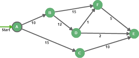
Given a positively weighted graph and a starting node (A), Dijkstra determines the shortest path and distance from the source to all destinations in the graph:
The core idea of the Dijkstra algorithm is to continuously eliminate longer paths between the starting node and all possible destinations.
To keep track of the process, we need to have two distinct sets of nodes, settled and unsettled.
Settled nodes are the ones with a known minimum distance from the source. The unsettled nodes set gathers nodes that we can reach from the source, but we don’t know the minimum distance from the starting node.
Here’s a list of steps to follow in order to solve the SPP with Dijkstra:
- Set distance to startNode to zero.
- Set all other distances to an infinite value.
- We add the startNode to the unsettled nodes set.
- While the unsettled nodes set is not empty we:
- Choose an evaluation node from the unsettled nodes set, the evaluation node should be the one with the lowest distance from the source.
- Calculate new distances to direct neighbors by keeping the lowest distance at each evaluation.
- Add neighbors that are not yet settled to the unsettled nodes set.
These steps can be aggregated into two stages, Initialization and Evaluation. Let’s see how does that apply to our sample graph:
2.1. Initialization
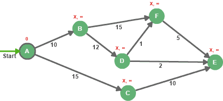
Before we start exploring all paths in the graph, we first need to initialize all nodes with an infinite distance and an unknown predecessor, except the source.
As part of the initialization process, we need to assign the value 0 to node A (we know that the distance from node A to node A is 0 obviously)
So, each node in the rest of the graph will be distinguished with a predecessor and a distance:
To finish the initialization process, we need to add node A to the unsettled nodes set it to get picked first in the evaluation step. Keep in mind, the settled nodes set is still empty.
2.2. Evaluation
Now that we have our graph initialized, we pick the node with the lowest distance from the unsettled set, then we evaluate all adjacent nodes that are not in settled nodes:
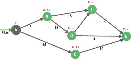
The idea is to add the edge weight to the evaluation node distance, then compare it to the destination’s distance. e.g. for node B, 0+10 is lower than INFINITY, so the new distance for node B is 10, and the new predecessor is A, the same applies to node C.
Node A is then moved from the unsettled nodes set to the settled nodes.
Nodes B and C are added to the unsettled nodes because they can be reached, but they need to be evaluated.
Now that we have two nodes in the unsettled set, we choose the one with the lowest distance (node B), then we reiterate until we settle all nodes in the graph:
Here’s a table that summarizes the iterations that were performed during evaluation steps:
| Iteration | Unsettled | Settled | EvaluationNode | A | B | C | D | E | F |
|---|---|---|---|---|---|---|---|---|---|
| 1 | A | – | A | 0 | A-10 | A-15 | X-∞ | X-∞ | X-∞ |
| 2 | B, C | A | B | 0 | A-10 | A-15 | B-22 | X-∞ | B-25 |
| 3 | C, F, D | A, B | C | 0 | A-10 | A-15 | B-22 | C-25 | B-25 |
| 4 | D, E, F | A, B, C | D | 0 | A-10 | A-15 | B-22 | D-24 | D-23 |
| 5 | E, F | A, B, C, D | F | 0 | A-10 | A-15 | B-22 | D-24 | D-23 |
| 6 | E | A, B, C, D, F | E | 0 | A-10 | A-15 | B-22 | D-24 | D-23 |
| Final | – | ALL | NONE | 0 | A-10 | A-15 | B-22 | D-24 | D-23 |
The notation B-22, for example, means that node B is the immediate predecessor, with a total distance of 22 from node A.
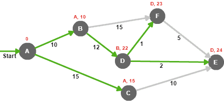
Finally, we can calculate the shortest paths from node A are as follows:
- Node B : A –> B (total distance = 10)
- Node C : A –> C (total distance = 15)
- Node D : A –> B –> D (total distance = 22)
- Node E : A –> B –> D –> E (total distance = 24)
- Node F : A –> B –> D –> F (total distance = 23)
3. Java Implementation
In this simple implementation we will represent a graph as a set of nodes:
public class Graph {

    private Set<Node> nodes = new HashSet<>();

    public void addNode(Node nodeA) {
        nodes.add(nodeA);
    }

    // getters and setters
}
A node can be described with a name, a LinkedList in reference to the shortestPath, a distance from the source, and an adjacency list named adjacentNodes:
public class Node {

    private String name;

    private List<Node> shortestPath = new LinkedList<>();

    private Integer distance = Integer.MAX_VALUE;

    Map<Node, Integer> adjacentNodes = new HashMap<>();

    public void addDestination(Node destination, int distance) {
        adjacentNodes.put(destination, distance);
    }

    public Node(String name) {
        this.name = name;
    }

    // getters and setters
}
The adjacentNodes attribute is used to associate immediate neighbors with edge length. This is a simplified implementation of an adjacency list, which is more suitable for the Dijkstra algorithm than the adjacency matrix.
As for the shortestPath attribute, it is a list of nodes that describes the shortest path calculated from the starting node.
By default, all node distances are initialized with Integer.MAX_VALUE to simulate an infinite distance as described in the initialization step.
Now, let’s implement the Dijkstra algorithm:
public static Graph calculateShortestPathFromSource(Graph graph, Node source) {
    source.setDistance(0);

    Set<Node> settledNodes = new HashSet<>();
    Set<Node> unsettledNodes = new HashSet<>();

    unsettledNodes.add(source);

    while (unsettledNodes.size() != 0) {
        Node currentNode = getLowestDistanceNode(unsettledNodes);
        unsettledNodes.remove(currentNode);
        for (Entry < Node, Integer> adjacencyPair:
          currentNode.getAdjacentNodes().entrySet()) {
            Node adjacentNode = adjacencyPair.getKey();
            Integer edgeWeight = adjacencyPair.getValue();
            if (!settledNodes.contains(adjacentNode)) {
                calculateMinimumDistance(adjacentNode, edgeWeight, currentNode);
                unsettledNodes.add(adjacentNode);
            }
        }
        settledNodes.add(currentNode);
    }
    return graph;
}
The getLowestDistanceNode() method, returns the node with the lowest distance from the unsettled nodes set, while the calculateMinimumDistance() method compares the actual distance with the newly calculated one while following the newly explored path:
private static Node getLowestDistanceNode(Set < Node > unsettledNodes) {
    Node lowestDistanceNode = null;
    int lowestDistance = Integer.MAX_VALUE;
    for (Node node: unsettledNodes) {
        int nodeDistance = node.getDistance();
        if (nodeDistance < lowestDistance) {
            lowestDistance = nodeDistance;
            lowestDistanceNode = node;
        }
    }
    return lowestDistanceNode;
}
private static void CalculateMinimumDistance(Node evaluationNode,
Integer edgeWeigh, Node sourceNode) {
Integer sourceDistance = sourceNode.getDistance();
if (sourceDistance + edgeWeigh < evaluationNode.getDistance()) {
evaluationNode.setDistance(sourceDistance + edgeWeigh);
LinkedList<Node> shortestPath = new LinkedList<>(sourceNode.getShortestPath());
shortestPath.add(sourceNode);
evaluationNode.setShortestPath(shortestPath);
}
}Now that all the necessary pieces are in place, let’s apply the Dijkstra algorithm on the sample graph being the subject of the article:
Node nodeA = new Node("A");
Node nodeB = new Node("B");
Node nodeC = new Node("C");
Node nodeD = new Node("D");
Node nodeE = new Node("E");
Node nodeF = new Node("F");

nodeA.addDestination(nodeB, 10);
nodeA.addDestination(nodeC, 15);

nodeB.addDestination(nodeD, 12);
nodeB.addDestination(nodeF, 15);

nodeC.addDestination(nodeE, 10);

nodeD.addDestination(nodeE, 2);
nodeD.addDestination(nodeF, 1);

nodeF.addDestination(nodeE, 5);

Graph graph = new Graph();

graph.addNode(nodeA);
graph.addNode(nodeB);
graph.addNode(nodeC);
graph.addNode(nodeD);
graph.addNode(nodeE);
graph.addNode(nodeF);

graph = Dijkstra.calculateShortestPathFromSource(graph, nodeA);
After calculation, the shortestPath and distance attributes are set for each node in the graph, we can iterate through them to verify that the results match exactly what was found in the previous section.
4. Conclusion
In this article, we’ve seen how the Dijkstra algorithm solves the SPP, and how to implement it in Java.