Weighted vs. Unweighted Graphs | Baeldung on Computer Science

1. Introduction

In this tutorial, we’ll talk about weighted and unweighted graphs. We’ll explain how they differ and show how we can represent them in computer programs.

2. What Is a Graph?

A graph is a collection of connected objects. They can be anything from purely mathematical concepts to real-world objects and phenomena. For example, a collection of people with family ties is a graph. So is a set of cities interconnected with roads.

Usually, we refer t0 the graph’s objects as nodes or vertices and to the connections between them as edges or arcs. For example, this is how we’d visualize a graph of cities and roads:

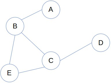
Each node represents a city, and each edge denotes a road from one city to another.

3. Unweighted Graphs

If we care only if two nodes are connected or not, we call such a graph unweighted. For the nodes with an edge between them, we say they are adjacent or neighbors of one another.

3.1. Adjacency Matrix

We can represent an unweighted graph with an adjacency matrix. It’s an $n\times n$ matrix consisting of zeros and ones, where $n$ is the number of nodes. If its element $a_{ij}$ is 1, that means that there’s an edge between the $i$ -th and $j$ -th nodes. If $a_{ij}=0$ , then there’s no edge between the two nodes.

This is how the adjacency matrix of the above roadmap graph would look like:

$\bordermatrix{ & A & B & C & D & E \cr A & 0 & 1 & 0 & 0 & 0 \cr B & 1 & 0 & 1 & 0 & 1 \cr C & 0 & 1 & 0 & 1 & 1 \cr D & 0 & 0 & 1 & 0 & 0 \cr E & 0 & 1 & 1 & 0 & 0 }$

It’s symmetrical, as is the case with all undirected graphs.

The matrix representation has two assumptions:

It is possible to map from the nodes to integers and assign a unique integer number to every node. (In our example: $A \mapsto 1, B \mapsto 2, C \mapsto 3, D \mapsto 4, E \mapsto 5$ .)
The number of nodes is such that the memory is big enough to reserve the consecutive space for an $n\times n$ matrix.

When those assumptions don’t hold or the graph is sparse, we use adjacency lists.

3.2. Adjacency Lists

For each node, we maintain a linked list of its neighbors:

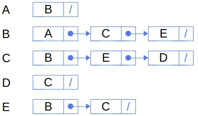
The main advantage of this representation is that the space for storing the graph need not be consecutive. However, we lose a very useful property of matrix representation, and that’s the $O(1)$ access complexity.

We can read the information on the adjacency of $i$ -th and $j$ -th nodes by accessing $a_{i,j}$ in a constant time, no matter the values of $i$ and $j$ . With linked lists, we may traverse the whole list. In the worst case, the $i$ -th node is a neighbor to all the vertices but the $j$ -th vertex from our query. So, we’ll check $n-2 \in O(n)$ items in the linked list to conclude that the two nodes aren’t connected.

4. Weighted Graphs

The unweighted graphs tell us only if two nodes are linked. So, they’re suitable for queries such as:

Is there a path between the nodes $u$ and $v$ ?
Which nodes are reachable from $u$ ?
How many nodes are on the shortest path between $u$ and $v$ ?

However, in many applications, the edges have numerical properties that we need to exploit in our algorithms to solve the problem at hand. For example, we must consider road lengths and traffic density while looking for the shortest path between two cities. So, we associate each edge $e$ with a real value $w(e)$ that we call its weight. We call such graphs weighted.

This is how the roadmap graph looks like when we include the edge weights, that is, the lengths of the roads:

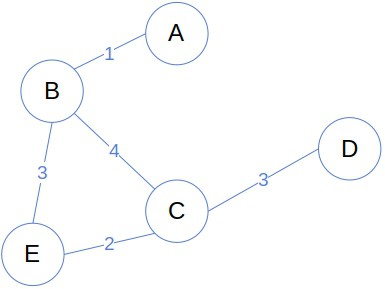
Just as nodes, the weights can be anything relevant for the problem at hand: lengths, densities, duration, costs, probabilities, and so on.

4.1. Representation of Weighted Graphs

The ways to represent weighted graphs are extensions of the unweighted graph’s representations.

The weight matrix $\boldsymbol{W=[w_{ij}]_{n\times n}}$ is a real matrix whose element $\boldsymbol{w_{ij}}$ represents the weight of the edge between the $\boldsymbol{i}$ -th and $\boldsymbol{j}$ -th nodes:

$\bordermatrix{ & A & B & C & D & E \cr A & 0 & 1 & 0 & 0 & 0 \cr B & 1 & 0 & 4 & 0 & 3 \cr C & 0 & 4 & 0 & 3 & 2 \cr D & 0 & 0 & 3 & 0 & 0 \cr E & 0 & 3 & 3 & 0 & 0 }$

The weights of actual edges are usually positive, so zero denotes that no edge exists between two nodes. However, if our application is such, the weights could be negative. In that case, we’ll have to define a special symbol that would indicate the absence of an edge in the matrix.

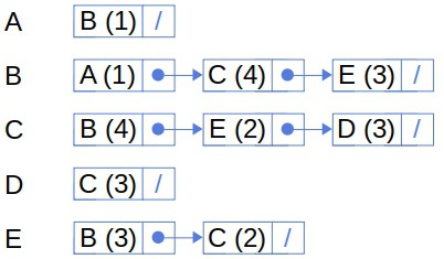
If we represent our graph via linked lists, we’ll have to store the edge weights alongside the neighbors in those lists:

4.2. Unweighted Graphs as Special Cases of Weighted Ones

Even the unweighted graphs can be considered weighted but with a special weight function $w$ :

$w(u, v) = \begin{cases} 0, & u \text{ and } v \text{ aren't connected} \\ 1, & u \text{ and } v \text{ are connected} \end{cases}$

Moreover, if the weights are all the same or the cost of a path depends only on the number of nodes it passes through, and we have the formula to calculate it, we don’t have to use the weighted representation. We can run the graph algorithms on the adjacency matrix and derive the solution with weights afterward.

4.3. Explicit vs. Implicit Graphs

Both weighted and unweighted graphs can be explicit or implicit. The explicit graphs are those whose nodes and edges we can enumerate and store in main or secondary memory, provided there’s enough space. So, before we run any algorithm on them, the explicit graphs are constructed in their entirety. The graph of cities and roads is an example of an explicit graph.

However, the graphs are sometimes so large or complicated that we can’t construct them in advance. Instead, we have a procedure that grows the graph as we explore it and constructs only the parts we need. Such graphs are known as implicit ones. We often use them in AI, where many search problems have infinite search spaces. Each candidate solution is a node in the search graph at hand, and when we want to find the neighboring solutions, we use a function that computes the neighbors on the fly.

The difference between the explicit and implicit graphs is analogous to that between eager and lazy loading.

5. Conclusion

In this article, we talked about the unweighted and weighted graphs. A graph of the former type is suitable for applications where we need to know only if two objects are directly connected via an edge. The latter we use when the edges have associated weights, such as costs, lengths, and similar.

Learn Java Collections

Learn Spring

Learn Maven

View All Courses

Core Concepts

Operating Systems

Neural Networks

Graph Theory

Latex

Full Archive

About Baeldung