

Learn through the super-clean Baeldung Pro experience:
>> Membership and Baeldung Pro.
No ads, dark-mode and 6 months free of IntelliJ Idea Ultimate to start with.
Learn through the super-clean Baeldung Pro experience:
>> Membership and Baeldung Pro.
No ads, dark-mode and 6 months free of IntelliJ Idea Ultimate to start with.
In this tutorial, we’ll investigate the effects of feature scaling in the Support Vector Machine (SVM).
First, we’ll learn about SVM and feature scaling. Then, we’ll illustrate the effect of feature scaling in SVM with an example in Python. Lastly, we conclude by comparing the classifier success.
SVM is a supervised learning algorithm we use for classification and regression tasks. It is an effective and memory-efficient algorithm that we can apply in high-dimensional spaces.
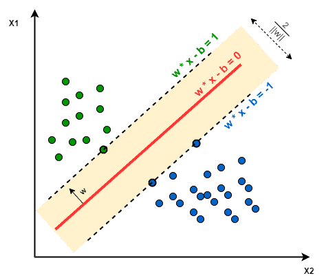
Training an SVM classifier includes deciding on a decision boundary between classes. This boundary is known to have the maximum distance from the nearest point on each data class. Due to this property, SVM is also referred to as a maximum-margin classifier:
SVM doesn’t implicitly support multi-class classification. We use one-vs-one or one-vs-rest approaches to train a multi-class SVM classifier.
Feature scaling is mapping the feature values of a dataset into the same range. Feature scaling is crucial for some machine learning algorithms, which consider distances between observations because the distance between two observations differs for non-scaled and scaled cases.
As we’ve already stated, the decision boundary maximizes the distance to the nearest data points from different classes. Hence, the distance between data points affects the decision boundary SVM chooses. In other words, training an SVM over the scaled and non-scaled data leads to the generation of different models.
The two most widely adopted approaches for feature scaling are normalization and standardization. Normalization maps the values into the [0, 1] interval:
![\[z = \frac{x - min(x)}{max(x) - min(x)}\]](/wp-content/ql-cache/quicklatex.com-9613d6dab45efff839236cb185a61e49_l3.svg "Rendered by QuickLaTeX.com")
Standardization shifts the feature values to have a mean of zero, then maps them into a range such that they have a standard deviation of 1:
![\[z = \frac{x - \mu}{\sigma}\]](/wp-content/ql-cache/quicklatex.com-355df7598ff32d0ae9a791830d67d6ab_l3.svg "Rendered by QuickLaTeX.com")
It centers the data, and it’s more flexible to new values that are not yet seen in the dataset. That’s why we prefer standardization in general.
Now that we’ve studied the theoretical concepts, let’s see how we can implement this in Python. We’ll utilize functions from the scikit learn library for preprocessing and model building.
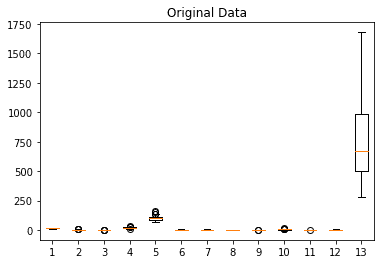
We’ll work with the wine dataset to train the model. The data is generated by chemical analysis of three types of wines. In this dataset, we have 13 real-valued features and three output classes.
The numerical features cover values in different ranges. Let’s visualize the input data with a boxplot:
Then, let’s train an SVM with the default parameters and no feature scaling. The SVC classifier we apply handles multi-class according to a one-vs-one scheme:
clf = svm.SVC()
clf.fit(X_train, y_train)
Next, we predict the outcomes of the test set:
y_pred = clf.predict(X_test)Afterward, let’s calculate the accuracy and the F-1 score metrics to measure the classification performance:
print("Accuracy:", metrics.accuracy_score(y_test, y_pred))
print("F-1 Score:", metrics.f1_score(y_test, y_pred, average=None))
Which gives the values:
Accuracy: 0.7592592592592593
F-1 Score: [1.         0.74509804 0.31578947]
So, the SVM model trained with default parameters has a 75% accuracy. F-1 Score values indicate that the prediction success for the classes is different: the first-class having perfect prediction accuracy, and the last class is the lowest.
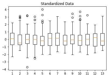
As an alternative approach, let’s train another SVM model with scaled features. We use the standard scaler to standardize the dataset:
scaler = StandardScaler().fit(X_train)
X_std = scaler.transform(X)
We need to always fit the scaler on the training set and then apply the transformation to the whole dataset. Otherwise, we’d leak some knowledge from the test set into the training set.
As expected, the resulting standardized features have a mean of 0 and a standard deviation of 1:
Then, let’s train a new model using the scaled data. The same code snippet used above works, we only change the input data.
The newly trained SVM model is completely different, as applying feature scaling changes the distances between data points. We can compare the model parameters to emphasize the difference. For example, n_support reports the number of support vectors for each class:
print(clf.n_support_)The first SVM model trained with the non-scaled dataset has the number of support vectors:
[15 34 34]whereas the second model trained on standardized data has:
[15 27 18]The numbers indicate that the second and third classes have different models.
Again, we compute the accuracy and the F-1 Scores to measure classification performance:
Accuracy: 0.9814814814814815
F-1 Score: [1.         0.97674419 0.96296296]
The new SVM model trained with standardized data has a much higher accuracy of 98%. Moreover, we observe a significant increase in the F-1 Score, especially for the third class.
The second and third classes having different F-1 Scores than the initial model verifies our observation with the number of support vectors. The models set up for these classes are not the same.
As a result, we see that feature scaling affects the SVM classifier outcome. Consequently, standardizing the feature values improves the classifier performance significantly.
In this article, we’ve learned about the SVM algorithm and how feature scaling affects its classification success.
After briefly describing the SVM and defining feature scaling, we’ve worked on a Python example to illustrate the difference.