

Yes, we're now running our only Summer Sale. All Courses are 30% off until 20th July, 2026:
Normalization vs Standardization in Linear Regression
Last updated: May 23, 2025
Learn through the super-clean Baeldung Pro experience:
>> Membership and Baeldung Pro.
No ads, dark-mode and 6 months free of IntelliJ Idea Ultimate to start with.
1. Introduction
In this tutorial, we’ll investigate how different feature scaling methods affect the prediction power of linear regression.
Firstly, we’ll learn about two widely adopted feature scaling methods. Then we’ll apply these feature scaling techniques to a toy dataset. Finally, we’ll compare and contrast the results.
2. Feature Scaling
In machine learning, feature scaling refers to putting the feature values into the same range. Scaling is extremely important for the algorithms considering the distances between observations like k-nearest neighbors. On the other hand, rule-based algorithms like decision trees are not affected by feature scaling.
A technique to scale data is to squeeze it into a predefined interval. In normalization, we map the minimum feature value to 0 and the maximum to 1. Hence, the feature values are mapped into the [0, 1] range:
![\[z = \frac{x - min(x)}{max(x) - min(x)}\]](/wp-content/ql-cache/quicklatex.com-9613d6dab45efff839236cb185a61e49_l3.svg "Rendered by QuickLaTeX.com")
In standardization, we don’t enforce the data into a definite range. Instead, we transform to have a mean of 0 and a standard deviation of 1:
![\[z = \frac{x - \mu}{\sigma}\]](/wp-content/ql-cache/quicklatex.com-355df7598ff32d0ae9a791830d67d6ab_l3.svg "Rendered by QuickLaTeX.com")
It not only helps with scaling but also centralizes the data.
In general, standardization is more suitable than normalization in most cases.
3. Feature Scaling in Python
To better illustrate the usage of feature scaling, let’s apply what we’ve learned so far. In Python, we can use the scikit-learn library for all machine learning tasks, including preprocessing.
In this section, we’ll work with the concrete compressive strength dataset. The regression problem is predicting concrete compressive strength, given quantities of seven components and the age of the concrete. There are 8 numerical input variables and 1030 instances in this dataset.
A box plot graphically shows the median, quartiles, and the range of numerical data. Let’s analyze the input features from the concrete compressive strength dataset with a boxplot:
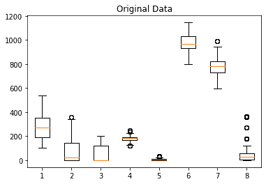
In the figure, we see the varying ranges of the input features. We also see where the majority of the data and the outliers are situated.
3.1. Normalization
For normalization, we utilize the min-max scaler from scikit-learn:
from sklearn.preprocessing import MinMaxScaler

min_max_scaler = MinMaxScaler().fit(X_test)
X_norm = min_max_scaler.transform(X)
As a rule of thumb, we fit a scaler on the test data, then transform the whole dataset with it. By doing this, we completely ignore the test dataset while building the model.
Normalizing the concrete dataset, we get:
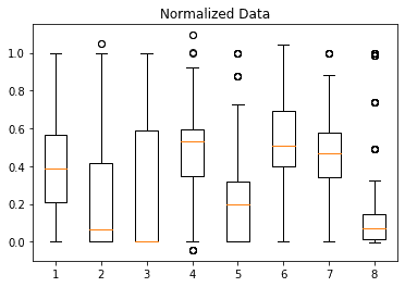
As promised, all values from various domains are transformed into the [0, 1] range. Careful observation on the last feature shows that extreme outlier values force the majority of observed values into an even smaller range. Moreover, the extreme outlier values in the new observations will be lost.
3.2. Standardization
To standardize a feature, we use the standard scaler:
from sklearn.preprocessing import StandardScaler

scaler = StandardScaler().fit(X_train)
X_std = scaler.transform(X)
Again, we fit the scaler using only the observations from the test dataset. The boxplot resulting from standardizing the concrete dataset shows how features are affected:
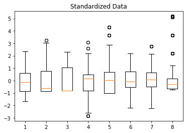
Let’s again observe the 8th feature. The outliers don’t affect how the majority of the values are transformed. Furthermore, the extreme values in the new observations will still be represented.
Before moving further, let’s visually compare how normalization and standardization change the data. To do so, let’s plot the 4th feature versus the 5th:
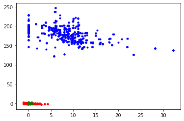
Blue dots represent the actual values of the input features. Red dots are the standardized values, and the green ones are the normalized values. As expected, normalization pushes data points close together. The resulting range is very small compared to the standardized dataset.
4. Linear Regression in Python
Now that we’ve learned how to apply feature scaling, we can move on to training the machine learning model. Let’s build a linear regression model:
from sklearn import linear_model

# Create linear regression object
regr = linear_model.LinearRegression()

# Train the model using the training sets
regr.fit(X_train, y_train)

# Make predictions using the testing set
y_pred = regr.predict(X_test)
After training the model, we can report the intercept and the coefficients:
# The intercept
print('Interccept: \n', regr.intercept_)
# The coefficients
print('Coefficients: \n', regr.coef_)
In our example, the output would be:
Intercept:
 -59.61868838556004
Coefficients:
 [ 0.12546445  0.11679076  0.09001377 -0.09057971  0.39649115  0.02810985
  0.03637553  0.1139419 ]
Furthermore, we can report the mean squared error, and R squared metrics:
print('MSE: %.2f' % mean_squared_error(y_test, y_pred))
print('R^2: %.2f' % r2_score(y_test, y_pred))
This gives the scores:
MSE: 109.75
R^2: 0.59
To train a linear regression model on the feature scaled dataset, we simply change the inputs of the fit function.
In a similar fashion, we can easily train linear regression models on normalized and standardized datasets. Then, we use this model to predict the outcomes for the test set and measure their performance.
For the concrete dataset, the results are:
| Linear Regression | MSE | R2 |
|---|---|---|
| Original Dataset | 109.75 | 0.59 |
| Normalized Data | 109.75 | 0.59 |
| Standardalized Data | 109.75 | 0.59 |
Surprisingly, feature scaling doesn’t improve the regression performance in our case. Actually, following the same steps on well-known toy datasets won’t increase the model’s success.
However, this doesn’t mean feature scaling is unnecessary for linear regression. Even the sci-kit implementation has a boolean normalize parameter to automatically normalize the input when set to True.
Instead, this result reminds us that there’s no fit for all preprocessing methods in machine learning. We need to carefully examine the dataset and apply customized methods.
5. Conclusion
In this article, we’ve examined two well-known feature scaling methods: normalization and standardization. We applied these methods in python to see how they transform the features of the concrete compressive strength dataset.
Then, we’ve trained linear regression models with this dataset as well as its normalized and standardized copies. In our example, this didn’t change the model’s success.