

Yes, we're now running our only Summer Sale. All Courses are 30% off until 20th July, 2026:
Learn through the super-clean Baeldung Pro experience:
>> Membership and Baeldung Pro.
No ads, dark-mode and 6 months free of IntelliJ Idea Ultimate to start with.
1. Introduction
In this tutorial, we’ll explore the concepts of precision and average precision in machine learning (ML). Both are performance metrics for classification, but although their names are similar, the difference is fundamental.
To keep things simple, we’ll focus on binary classification, where we have only two classes: one positive and the other negative.
2. Classification Performance Metrics
When testing ML classifiers, we’re interested in several metrics, including but not limited to accuracy, the  score, and AUROC. In binary classification, those metrics evaluate our classifier’s capacity to differentiate between two classes.
To compute the metrics, we use four basic scores:
| Predicted positive | Predicted negative | |
|---|---|---|
| Actually positive | TP | FN |
| Actually negative | FP | TN |
In the table,  is the number of true positives,
  denotes the number of false positives,
  is the number of true negatives, and
  stands for the number of false negatives.
3. Precision
Precision is the ratio of correctly predicted positives and predicted positives. More specifically, precision tells us how many objects we classify as positive belong to the positive class.
For instance, let’s say that our classifier labeled 150 objects as positive and that TP is 120. Then, the classifier’s precision is:
![\[\frac{120}{150} = \frac{4}{5} = 80\%\]](/wp-content/ql-cache/quicklatex.com-0375ebdd40c765634ed66a2ebd0f10c9_l3.svg "Rendered by QuickLaTeX.com")
From the example, we see that the formula for precision is:
(1) 
We can interpret it as the probability that the assigned positive label is correct. That explains the metric’s name: it quantifies how precise the (positive) predictions are.
4. Average Precision
Precision describes a specific ML classifier. In contrast, the average precision evaluates a family of classifiers. To explain the difference, let’s first formalize the notion of threshold-based binary classifiers.
4.1. Threshold-based Binary Classifiers
We can define many binary classifiers as indicator functions:
(2) 
where  is the score the classifier computes for the object
  before classifying it, which denotes the confidence with which the classifier can label as positive, and
  is the decision threshold. So, higher values of correspond to a higher confidence that is positive, and vice versa.
For instance, in Support Vector Machines, is the signed distance to separating hyperplane, and  . In Logistic Regression models, estimates the probability that is positive, and
  .
.
So, the precision as we calculate it using Equation (1) is a function of , just as and :
(3) 
4.2. The Average Precision Metric
By varying , we get a family of classifiers having the same form. If we calculate the precision at each and then compute the mean, we get the average precision (AP):
(4) 
where  are chosen thresholds. Such defined
  estimates the expected precision with respect to the distribution of the thresholds. Assuming that they’re uniformly distributed between
  and
and  , we get the formula for the expected precision:
(5) 
So, to get a precise and unbiased estimate, we need to use enough thresholds and cover the range evenly.
5. Average Precision in the Precision-Recall Space
There’s a problem with the average precision defined above. First, thresholds can have different, even unbounded ranges (when  or
or  or both).
For that reason, a visual comparison of the classifiers with different ranges may be difficult or impossible. For example, the  -scores, and consequently, the thresholds , are unbounded in Support Vector Machines, so we have to cover the whole
  on the -axis. In contrast, the scores belong to
 ![[0, 1]](/wp-content/ql-cache/quicklatex.com-944fdd98d4f1854c8720f98d8b20b6ad_l3.svg "Rendered by QuickLaTeX.com") in Logistic Regression. The difference in scales means that we can’t compare the two precision curves easily:
in Logistic Regression. The difference in scales means that we can’t compare the two precision curves easily:
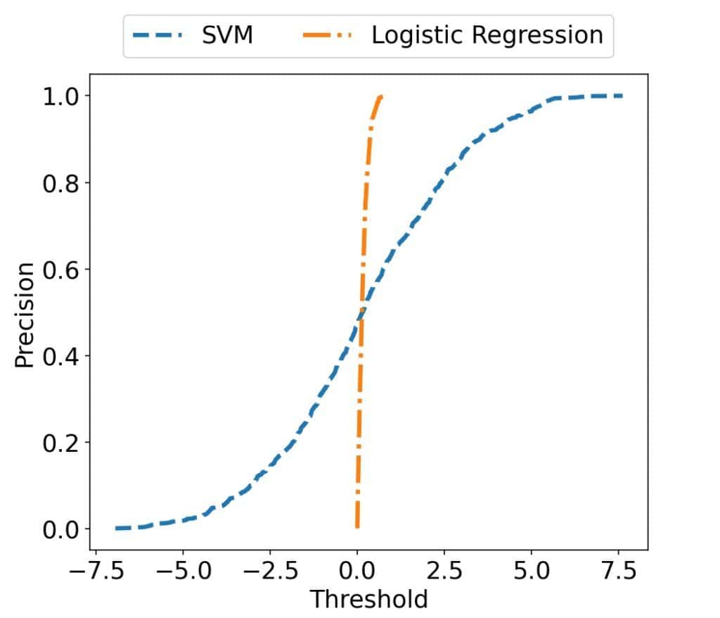
When we analyze the plot, it isn’t clear which classifier family works better.
Second, this version of AP doesn’t consider the recall.
It turns out that we can address both issues in the precision-recall (PR) space. So, let’s quickly revise what the recall is and why it’s important.
5.1. Recall
In contrast to precision, the recall score tells us how many positive objects our classifier correctly identifies as positive. So, we define and compute it as the ratio of true positives and the total number of positive objects in our data:
(6) 
The difference between the two metrics is subtle but critical. Recall estimates a classifier’s ability to label all positive objects as such. Precision estimates the ability to identify only positive objects as positive.
5.2. Weighted Average Precision
If we considered only precision, we could get a good score by classifying as positive only the objects with a high -value. That would result in an overly conservative classifier failing to identify many positive objects. So, it wouldn’t be useful in practice due to a low recall.
Therefore, we want a metric that considers both scores. Since we’d like to have both precision and recall high, we could incorporate the latter into the formula for the average precision by multiplying each  with the realized recall gain.
So, if  and
and  , our adjusted average precision is:
(7) 
5.3. Geometry
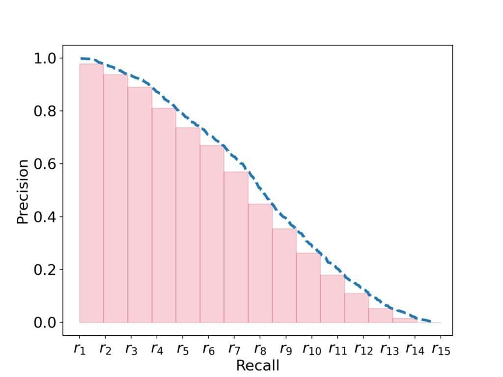
The AP from Formula (7) has a nice visual interpretation in the PR space.
Let the -axis denote recall, and let the  -axis represent precision. Then, the AP (7) estimates the area under the precision curve in the PR space:
Further, since recall and precision take values from ![\boldsymbol{[0, 1]}](/wp-content/ql-cache/quicklatex.com-efa1faca843512d7d149bf8fe06168d0_l3.svg "Rendered by QuickLaTeX.com") , we can visualize the precision curves of different classifiers on the same plot in a way that allows for direct comparison. For example, let’s take a look at the curves of the SVM and LR models from above, but now in the PR space:
, we can visualize the precision curves of different classifiers on the same plot in a way that allows for direct comparison. For example, let’s take a look at the curves of the SVM and LR models from above, but now in the PR space:
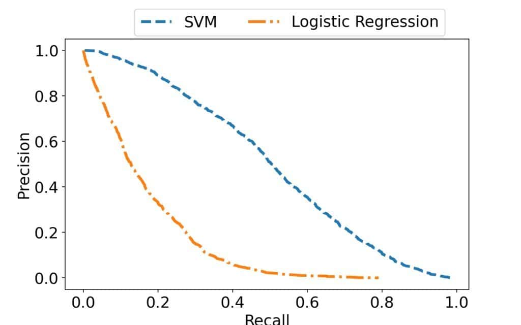
Since the x-axis ranges are the same, the difference is now easy to spot.
6. A Word of Caution
Since precision and recall don’t consider negative objects, we can use the precision and average precision scores when false negatives can be ignored.
However, if true negatives add value, we shouldn’t overlook them. Instead, we should calculate the scores that take both classes into account.
7. Conclusion
In this article, we talked about precision and average precision. The former evaluates a specific classifier, whereas the latter describes the performance of a classifier family.