

Learn through the super-clean Baeldung Pro experience:
>> Membership and Baeldung Pro.
No ads, dark-mode and 6 months free of IntelliJ Idea Ultimate to start with.
Last updated: February 12, 2025
Learn through the super-clean Baeldung Pro experience:
>> Membership and Baeldung Pro.
No ads, dark-mode and 6 months free of IntelliJ Idea Ultimate to start with.
Recurrent Neural Networks (RNNs) are well-known networks capable of processing sequential data. Closely related are Recursive Neural Networks (RvNNs), which can handle hierarchical patterns.
In this tutorial, we’ll review RNNs, RvNNs, and their applications in Natural Language Processing (NLP). Also, we’ll go over some of those models’ advantages and disadvantages for NLP tasks.
RNNs are a class of neural networks that can represent temporal sequences, which makes them useful for NLP tasks because linguistic data such as sentences and paragraphs have sequential nature.
Let’s imagine a sequence  of an arbitrary length.
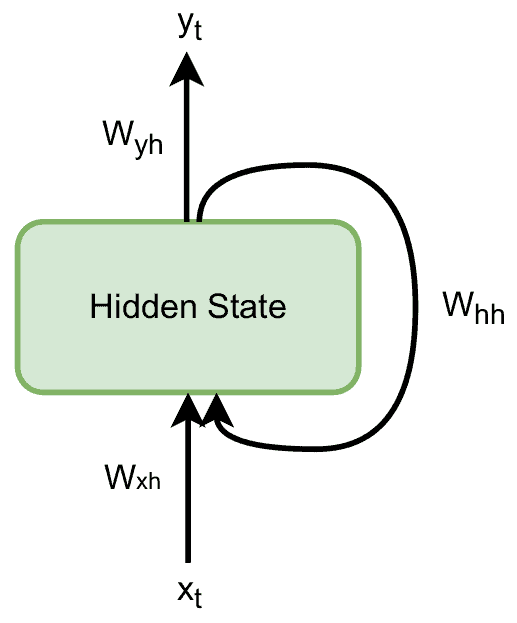
An RNN processes the sequence one element at a time, in the so-called time steps. At step  , it produces the output
  and has the hidden state
  , which serves as the representation of the subsequence
  .
.
The RNN calculates the hidden state by combining  and
and  . It multiplies them with matrices
  and
and  and applies the transformation
  to the sum:
![\[ h_t = f_W(W_{hh}h_{t-1} + W_{xh}x_{t-1}) \]](/wp-content/ql-cache/quicklatex.com-14b3d9a8ef3f4f254955110002e1cab0_l3.svg "Rendered by QuickLaTeX.com")
Then, the output is the product of the matrix  and :
and :
![\[ y_t = W_{yh}h_t \]](/wp-content/ql-cache/quicklatex.com-4ecfbf93785e5e9496cd70f4273b443a_l3.svg "Rendered by QuickLaTeX.com")
Since the matrices are the same across the steps, the network has a simple diagram:
Training the network consists of learning the transformation matrices. A widely used algorithm that does that well is the Gradient Descent algorithm.
Usually, we initialize the weights and the first hidden state randomly. For the function , there are several alternatives. For example, we can go with the  function:
![\[ \tanh (z) = \frac{e^{2z} - 1}{e^{2z} + 1} \]](/wp-content/ql-cache/quicklatex.com-4e57192b4ffe8ff6e3cd0d0a72d3d498_l3.svg "Rendered by QuickLaTeX.com")
As an example, we can take a look at an encoder-decoder model for machine translation. In this scenario, the encoder receives a sentence in the original language, and the decoder produces the translation in the target language. Let’s imagine that our original language is English and the target language is Spanish:
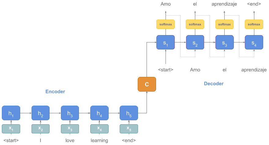
We can use RNNs for both the encoder and decoder parts of our machine-translation system. Although the number of words in each sentence may vary, an RNN processes a sequence until reaching the end token no matter how long the sequence is. So, we see an advantage of RNNs in action.
The advantages of RNNs are mainly threefold. The first one is that they can process inputs of any length. This is in contrast to other networks such as CNNs that can process only fixed-length inputs. As a result, we can use RNNs with sequences that are short as well as very long without changing our network’s architecture.
The second benefit is that the hidden state acts like some type of memory. As the network processes the elements of a sequence one by one, the hidden state stores and combines the information on the whole sequence.
Finally, the third advantage of RNNs is that they share the weights across time steps. This allows the network to stay the same size (with the same number of parameters) for sequences of varying lengths.
We can also consider three drawbacks of RNNs. Firstly, due to their sequential nature, they can be slow to train. In other words, as the input to one step of the networks comes from the previous step, it is difficult to perform the steps in parallel to make the training faster.
Secondly, RNNs have a problem called vanishing or exploding gradients. The former problem occurs when multiplying many gradients less than one. The result is a near-zero value, so it doesn’t contribute to the weights update. The latter happens when we multiply many gradients larger than one, so the result explodes. A solution is to use non-linear activation functions such as ReLU that don’t result in small derivatives. In addition, other variants of RNNs, such as Long Short-Terms Memory (LSTM), address this issue.
The last problem is that vanilla RNNs can have difficulty processing the long-term dependencies in sequences. Long-term dependencies may happen when we have a long sequence. If two complementary elements in the sequence are far from each other, it can be hard for the network to realize they’re connected. For instance, let’s consider this sequence:
Programming is a lot of fun and exciting especially when you’re interested in teaching machines what to do. I’ve seen many people from five-year-olds to ninety-year-olds learn it.
Here, the word it at the end of the sentence refers to programming which is the first word. In between, there are many other words, which could cause an RNN to miss the connection. This happens even though RNNs have some type of memory. However, the LSTMs can resolve this issue.
RvNNs generalize RNNs. Because of their tree structure, they can learn the hierarchical models as opposed to RNNs that can handle only sequential data. The number of children for each node in the tree is fixed so that it can perform recursive operations and use the same weights across the steps.
The tree structure of RvNNs means that to combine the child nodes and produce their parents, each child-parent connection has a weight matrix. Similar children share the same weights. In other words, considering a binary tree, all the right children share one weight matrix and all the left children share another weight matrix. In addition, we need an initial weight matrix ( ) to calculate the hidden state for each raw input:
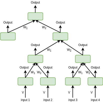
Therefore, the number of weight matrices is equal to the number of children that a node can have. We can calculate the parent node’s representation by summing the products of the weight matrices ( ) and the children’s representations (
 ) and applying the transformation
  :
:
![\[h = f \left( \sum_{i=1}^{i=c} W_i C_i \right) \]](/wp-content/ql-cache/quicklatex.com-ed10261a1277259164190d415366cc72_l3.svg "Rendered by QuickLaTeX.com")
where  is the number of children.
Training RvNNs is similar to RNNs with the same optimization algorithm. There’s a weight matrix for each child that the model needs to learn ( ). These weight matrices are shared across different recursions for the subsequent children at the same position.
One of the main applications of RvNNs in NLP is the syntactic parsing of natural language sentences.
When parsing a sentence, we want to identify its smaller components such as noun or verb phrases, and organize them in a syntactic hierarchy:
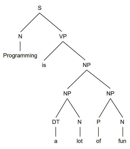
Since RNNs consider only sequential relations, they’re less suitable for handling hierarchical data in contrast compared to RvNNs. Let’s say that want to capture the representation of the phrase a lot of fun in this sentence:
Programming is a lot of fun.
What representation would an RNN give to this phrase? Since each state depends on the preceding words’ representation, we can’t represent a subsequence that doesn’t start at the beginning of the sentence. So, when our RNN processes the word fun, the hidden state at that time step will represent the entire sentence.
In contrast, the hierarchical architecture of RvNNs can store the representation of the exact phrase:
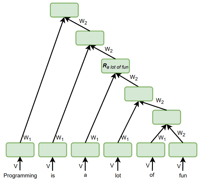
It is in the hidden state of the node  .
.
Two main advantages of RvNNs for NLP tasks are their structure and network depth reduction.
As we’ve seen, the tree structure of RvNNs can handle the hierarchical data, such as in the parsing problems.
Another RvNNs’ advantage is that the trees can have a logarithmic height. More specifically, when we have  input words, an RvNN can return a binary tree with height
  . Since this reduces the distance between the first and the last input elements, the long-term dependency becomes shorter and easier to catch.
The tree structure of RvNNs can also be a disadvantage. Using them means that we’re introducing a special inductive bias to our model. Here, the inductive bias is the assumption that the data follow a tree hierarchy. However, when that isn’t the case, the network may fail to learn the existing patterns.
Another problem with RvNNs is that parsing can be slow and ambiguous. In particular, there can be several parse trees for a single sentence.
In addition, labeling the training data for RvNNs is more time-consuming and labor-intensive than constructing RNNs. Manually parsing a sequence into smaller components takes considerably more time and effort than assigning a label to a sequence.
| When to use RNNs | When to use RvNNs |
|---|---|
| Sequential data | Hierarchical data |
| Inputs of variable lengths | A shallower network |
In this article, we explained the advantages and disadvantages of the recurrent (RNN) and recursive neural networks (RvNN) for Natural Language Processing.
The main difference is the type of patterns they can catch in data. While RNNs can process sequential data, RvNNs can find hierarchical patterns.