Encoder-Decoder Models for Natural Language Processing

1. Overview

Encoder-Decoder models and Recurrent Neural Networks are probably the most natural way to represent text sequences.

In this tutorial, we’ll learn what they are, different architectures, applications, issues we could face using them, and what are the most effective techniques to overcome those issues.

All the background required to understand it is basic knowledge about artificial neural networks and backpropagation.

2. Introduction

2.1. Encoders with Recurrent Neural Networks

Understanding text is an iterative process for humans: When we read a sentence, we process each word accumulating information up to the end of the text.

A system accumulating information composed of similar units repeated over time is a Recurrent Neural Network (RNN) in the Deep Learning field.

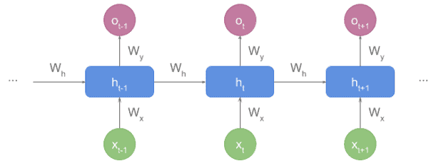
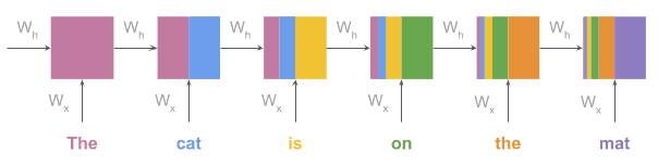
In general, a text encoder turns text into a numeric representation. This task can be implemented in many different ways but, in this tutorial, what we mean by encoders are RNN encoders. Let’s see a diagram:

Depending on the textbook, we can find it in rolled representation:

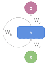
So each block is composed of the following elements at time ${t}$ :

Block Input:

Input Vector $\vec{x_t}$ (encoding the word)
Hidden state vector $\vec{h_{t-1}}$ (containing the sequence state before the current block)

Block Output:

Output vector $\vec{o_t}$ , which is not always produced by each block, as we’ll see in a few moments

Weights:

${W_x}$ weights between $\vec{x_t}$ and $\vec{h_t}$
${W_h}$ weights between $\vec{h_{t+1}}$ and $\vec{h_t}$
${W_x}$ weights between $\vec{h_t}$ and $\vec{o_t}$

2.2. Decoders

Unlike encoders, decoders unfold a vector representing the sequence state and return something meaningful for us like text, tags, or labels.

An essential distinction with encoders is that decoders require both, the hidden state and the output from the previous state.

When the decoder starts processing, there’s no previous output, so we use a special token <start> for those cases.

Let’s make it clearer with the example below, which shows how machine translation works:

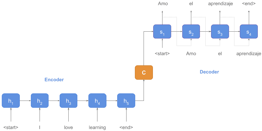
The encoder produced state ${C}$ representing the sentence in the source language (English): I love learning.

Then, the decoder unfolded that state ${C}$ into the target language (Spanish): Amo el aprendizaje.

${C}$ could be considered a vectorized representation of the whole sequence or, in other words, we could use an encoder as a rough mean to obtain embeddings from a text of arbitrary length, but this is not the proper way to do it, as we’ll see in another tutorial.

2.3. Further Details

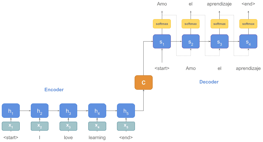
In the previous diagram, we used words as input for simplicity, but what we really pass is each word embeddings vector ( $\vec{x}_1$ , $\vec{x}_2$ , …)

Also, in the decoder part of the diagram, there should be a softmax function that finds the word from the vocabulary with the highest probability for that input and hidden state.

Let’s update our diagram with these additional details:

encoder decoder with embeddings softmax2

3. Architectures and Their Applications

3.1. Many to One

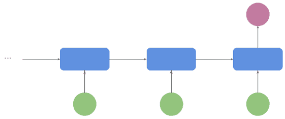
This is widely used for classification, typically sentiment analysis or tagging. The input is a sequence of words, and the output is a category. This output is produced by the last block of the sequence:

3.2. One to Many

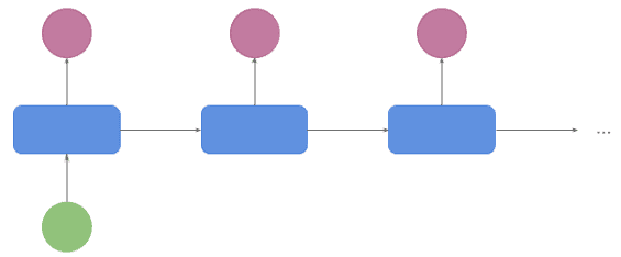
The main application of this architecture is text generation. The input is a topic, and the output is the sequence of words generated for that topic:

3.3. Many to Many (1st version)

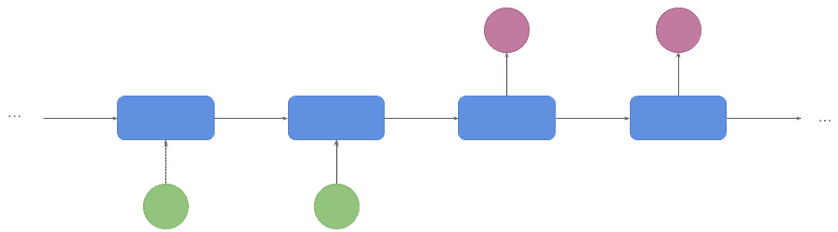
This is a very popular architecture in Machine Translation (also known as seq2seq). The input is a sequence of words, and so is the output.

The network “waits” for the encoding step to finish producing the internal state. It just starts decoding when the encoder finished:

3.4. Many to Many (2nd version)

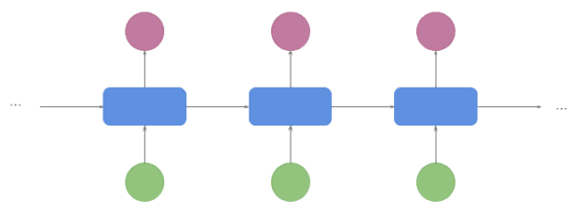
Common applications for this architecture are video captioning and part of speech tagging. At the same time the frames go, the captions/tags are produced, so there’s no waiting for a final state before decoding it:

4. Pros and Cons

The advantages of Recurrent Neural Networks are:

We can feed them inputs of any length
The model size doesn’t grow with the input size
They naturally model events over time

The disadvantages are the following:

They are slow because they must be processed sequentially. Bear in mind we always need the previous state to calculate the current one
There are vanishing and exploding gradient problems
They don’t perform well with long sequences

5. LSTM and GRU Units

5.1. What Are Vanishing/Exploding Gradients?

The gradient is that vector we use to update the network weights so it can perform better in the future.

Because of backpropagation and the chain rule, when the gradient update is small, it decreases exponentially with the number of layers. Therefore, in very deep architectures with lots of layers, an update happening at a very deep layer doesn’t have any effect on the front layers (it vanishes), and the network can’t learn.

In the picture below, we see an RNN where initial updates lose strength exponentially with the flow of the sequence:

We face the opposite situation with exploding gradients: If the gradient is big, it increases exponentially, making the learning process very unstable.

LSTM and GRU units were created to fix this kind of problem.

5.2. Basic RNN Units

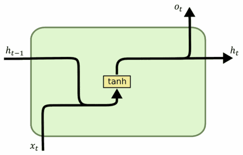
Vanilla RNN units look like this:

Input: The previous state in the sequence and the word vector for the current state
Output: Current state to be passed to the next unit and output vector

Let’s see how to code an RNN using vanilla units in Python and Tensorflow:

import tensorflow as tf

...

model = tf.keras.Sequential([
  tf.keras.layers.Embedding(vocab_size, 64),
  tf.keras.layers.GlobalAveragePooling1D(),
  tf.keras.layers.Dense(64, activation='relu'),
  tf.keras.layers.Dense(1, activation='sigmoid')
])

5.3. LSTM

Long short-term memory (LSTM) units are composed of a cell, an input gate, an output gate and a forget gate.

In the next picture we have a diagram of an LSTM:

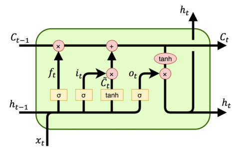
The function of each element composing this unit is:

Cell state: This is the state of the cell (the memory)
Input gate: It regulates how much a new value can flow into the cell
Forget gate: It controls to what extent a new value remains in the cell
Output gate: It regulates the extent to which the value in the cell is used to compute the output activation of the LSTM unit

By using these gates controlling long-term dependencies in the sequence, RNNs avoid some key information to be lost.

The code to create an RNN using LSTMs would be:

import tensorflow as tf

...

model = tf.keras.Sequential([
  tf.keras.layers.Embedding(vocab_size, 64),
  tf.keras.layers.Bidirectional(tf.keras.layers.LSTM(64)),
  tf.keras.layers.Dense(64, activation='relu'),
  tf.keras.layers.Dense(1, activation='sigmoid')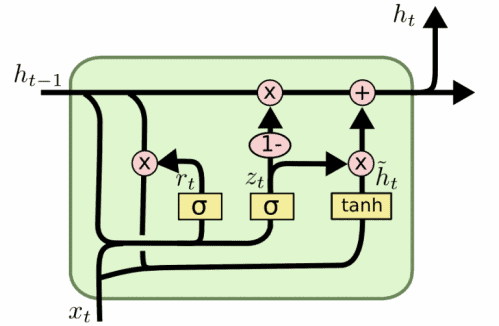
])

5.4. GRU

Gated recurrent units (GRU) are more recent and their design is similar to LSTMs, but using fewer parameters (they lack the output gate):

Let’s have a look at the code:

import tensorflow as tf

...

model = tf.keras.Sequential([
  tf.keras.layers.Embedding(vocab_size, 64),
  tf.keras.layers.Bidirectional(tf.keras.layers.GRU(64)),
  tf.keras.layers.Dense(64, activation='relu'),
  tf.keras.layers.Dense(1, activation='sigmoid')
])

5.5. When to Use Each?

In general, don’t use vanilla RNNs, always use LSTM or GRU units.

How to choose between LSTM or GRU? There’s no rule of thumb: it often depends on the task, so try both and use the best performing unit.

In case they perform similarly, prefer GRU over LSTM as they are less computationally expensive.

6. Attention Mechanism

LSTM and GRU improve RNN’s performance with longer sequences, but some specific tasks require even more power to work properly.

One typical example is neural machine translation, where grammar structures in the encoder and decoder are quite different. To translate each next word, we need to focus on specific words from the input sentence, possibly in a very different order.

Let’s see an example translating the sentence “L’accord sure la zone économique européene a été signé en août 1992″ into English:

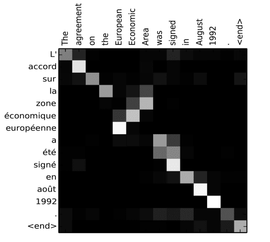
In the matrix above we can see how “zone” is focusing heavily on “Area”, and more softly on “Economic”. We can also notice how “européenne” is strongly focused on “European”.

What we see here is that the attention mechanism allows the decoder to focus on specific parts of the input sequence to properly produce the next output.

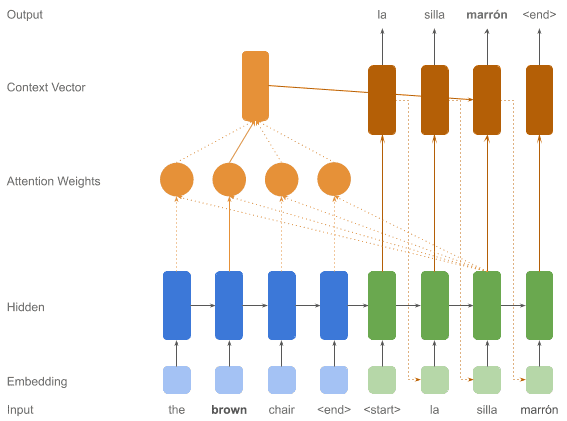
See below a diagram illustrating how this mechanism fits in the architecture we already had:

7. Conclusion

In this article, we studied the building blocks of encoder-decoder models with recurrent neural networks, as well as their common architectures and applications.

We also addressed the most frequent issues we’ll face when using these models and how to fix them by using LSTM or GRU units, and the attention mechanism.

Now that we learned all these new techniques, together with the provided helper code snippets, we’re ready to start creating our own models in real life.

Full Archive

About Baeldung

Core Concepts

Operating Systems

Artificial Intelligence

Graph Theory

Latex