Differences Between Bidirectional and Unidirectional LSTM

1. Introduction

In this tutorial, we’ll introduce one type of recurrent neural network that’s commonly used with a sequential type of data called long-short term memory (LSTM). This is surely one of the most commonly used recurrent neural networks. First, we’ll briefly introduce the terms of neural networks, as well as recurrent neural networks.

After that, we’ll dive deep into LSTM architecture and explain the difference between bidirectional and unidirectional LSTM. Finally, we’ll mention several applications for both types of networks.

2. Neural Networks

Neural networks are algorithms explicitly created as an inspiration for biological neural networks. The basis of neural networks is neurons interconnected according to the type of network. Initially, the idea was to create an artificial system that would function just like the human brain.

There are many types of neural networks, but they roughly fall into three main classes:

For the most part, the difference between them is the type of neurons that form them, and how the information flows through the network.

In this tutorial, we’ll only work with recurrent neural networks and LSTM in particular.

3. Recurrent Neural Networks

While in standard feedforward neural networks each input vector component has its weights, in recurrent networks, each component shares the same weights. Generally, the advantage of recurrent networks is that they share weights for each position of the input vector. Also, a model can process sequences with different lengths by sharing the weights. Another advantage is that it reduces the number of parameters (weights) that the network needs to learn.

The basic principle in recurrent networks is that the input vector and some information from the previous step (generally a vector) are used to calculate the output and information passed to the next step. In general, the formulas used to calculate the output values in each step are called units (blocks).

Thus, for the simplest recurrent network, one block can be defined by the relation:

(1) $\begin{align*} a^{<t>} &= f_{1}(W_{aa}a^{<t-1>} + W_{ax}x^{<t>} + b_{a})\\ \hat{y}^{<t>} &= f_{2}(W_{ya}a^{<t>} + b_{y}), \end{align*}$

$x^{<t>}$ is a vector or a number that’s part of an input sequence, $t$ indicates the step for calculating recurrent relations, $W_{aa}, W_{ax}, W_{ya}, b_{a}$ and $b_{y}$ are weight matrices and vectors with given dimension, and $f_{1}$ and $f_{2}$ are activation functions. Usually, for $f_{1}$ , we take $tanh$ or $ReLU$ , while for $f_{2}$ , since it calculates the output value, we take $sigmoid$ or $softmax$ . Finally, in the image below, we can observe the whole architecture of this block:

4. LSTM

LSTM is a special type of recurrent neural network. Specifically, this architecture is introduced to solve the problem of vanishing and exploding gradients. In addition, this type of network is better for maintaining long-range connections, recognizing the relationship between values at the beginning and end of a sequence.

The LSTM model introduces expressions, in particular, gates. In fact, there are three types of gates:

forget gate – controls how much information the memory cell will receive from the memory cell from the previous step
update (input) gate – decides whether the memory cell will be updated. Also, it controls how much information the current memory cell will receive from a potentially new memory cell.
output gate – controls the value of the next hidden state

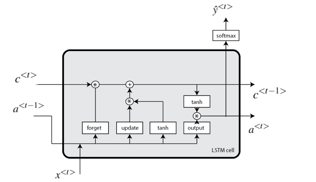
Mathematically, we define an LSTM block as:

(2) $\begin{align*} &\Gamma_{u} = \sigma(W_{uu}a^{<t-1>} + W_{ux}x^{<t>} + b_{u})\\ &\Gamma_{f} = \sigma(W_{ff}a^{<t-1>} + W_{fx}x^{<t>} + b_{f})\\ &\Gamma_{o} = \sigma(W_{oo}a^{<t-1>} + W_{ox}x^{<t>} + b_{o})\\ &\hat{c}^{<t>} = tanh(W_{cc}a^{<t-1>} + W_{cx}x^{<t>} + b_{c})\\ &c^{<t>} = \Gamma_{u}\odot \hat{c}^{<t>} + \Gamma_{f}\odot c^{<t-1>}\\ &a^{<t>} = \Gamma_{o}\odot \tanh(c^{<t>}), \end{align*}$

$W$ and $b$ are weight matrices and vectors, $t$ is the current iteration of the recurrent network, $\Gamma_{u}$ is the update gate, $\Gamma_{f}$ is the forget gate, $\Gamma_{o}$ is the output gate, $\hat{c}^{<t>}$ is the potential value of the memory cell, $c^{<t>}$ is the current value of the memory cell, and $a^{<t>}$ is the output value or hidden state. The architecture of the LSTM block can be shown as:

5. Bidirectional LSTM

Bidirectional LSTM (BiLSTM) is a recurrent neural network used primarily on natural language processing. Unlike standard LSTM, the input flows in both directions, and it’s capable of utilizing information from both sides. It’s also a powerful tool for modeling the sequential dependencies between words and phrases in both directions of the sequence.

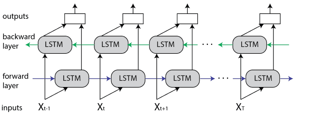
In summary, BiLSTM adds one more LSTM layer, which reverses the direction of information flow. Briefly, it means that the input sequence flows backward in the additional LSTM layer. Then we combine the outputs from both LSTM layers in several ways, such as average, sum, multiplication, or concatenation.

To illustrate, the unrolled BiLSTM is presented in the figure below:

5.1. Advantages

This type of architecture has many advantages in real-world problems, especially in NLP. The main reason is that every component of an input sequence has information from both the past and present. For this reason, BiLSTM can produce a more meaningful output, combining LSTM layers from both directions.

For example, the sentence:

Apple is something that…

might be about the apple as fruit or about the company Apple. Thus, LSTM doesn’t know what “Apple” means, since it doesn’t know the context from the future.

In contrast, most likely in both of these sentences:

Apple is something that competitors simply cannot reproduce.

and

Apple is something that I like to eat.

BiLSTM will have a different output for every component (word) of the sequence (sentence). As a result, the BiLSTM model is beneficial in some NLP tasks, such as sentence classification, translation, and entity recognition. In addition, it finds its applications in speech recognition, protein structure prediction, handwritten recognition, and similar fields.

Finally, regarding the disadvantages of BiLSTM compared to LSTM, it’s worth mentioning that BiLSTM is a much slower model and requires more time for training. Thus, we recommend using it only if there’s a real necessity.

6. Conclusion

In this article, we presented one recurrent neural network called BiLSTM. After an introduction to neural networks, we explained both the unidirectional and bidirectional LSTM algorithms in depth. In addition to the algorithmic differences between these methods, we mentioned key differences in their applications.

Full Archive

About Baeldung

Core Concepts

Operating Systems

Artificial Intelligence

Graph Theory

Latex