Intuition Behind Kernels in Machine Learning | Baeldung on Computer Science

1. Introduction

In this tutorial, we’ll explain the role of kernels in machine learning intuitively.

The so-called kernel trick enables us to apply linear models to non-linear data, which is the reason it has gained popularity in science and industry. In addition to classification, which is the task we usually associate them with, kernels can help us solve other problems in the field, such as regression, clustering, and dimensionality reduction..

2. Kernels Help When Linear Models Are Insufficient

Linear models are appealing for several reasons. First, the optimization problems we solve while training them have straightforward analytical solutions. Second, many would argue that linear models are inherently interpretable, so the users can understand how they work and the meaning of their components. They’re also easy to communicate and visualize. And, last but not least, they admit for a relatively simple mathematical analysis. For instance, such are Support Vector Machines, Linear Regression, and Principal Components Analysis.

However, linear models like those break down in the presence of non-linear relationships in the data. Let’s illustrate that with an example.

2.1. Example

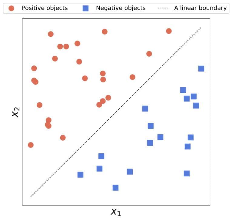
It’s easy to fit a straight line to reasonably linear data to find a linear boundary between linearly separable classes:

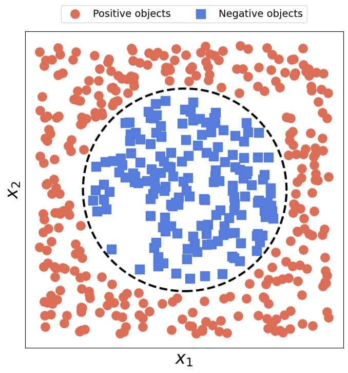
Unfortunately, no straight line can capture a circular boundary:

As a rule, the more complex and pronounced the non-linear relationships in the data are, the poorer the linear model’s performance. Still, we’d like to have models that keep the favorable properties of the linear ones but can handle arbitrarily complex data.

Kernels allow us precisely that. The idea is to map the data from the original space to a new one where they will be linear. For example, applying the transformation $\begin{bmatrix} x_1 \\ x_2 \end{bmatrix} \mapsto \begin{bmatrix} x_1 \\ x_2 \\ \sqrt{x_1^2 + x_2^2} \end{bmatrix}$ to the circular dataset, we get linearly separable data:

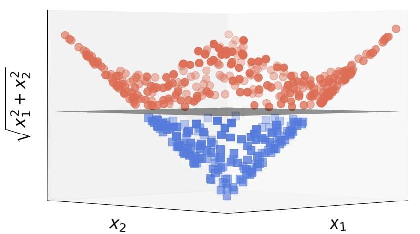
Kernels can make data linearly separable

As we see, the circular boundary in the original space becomes a plane in the transformed one.

3. The Mathematics of Kernels

How do the kernels work? Well, we said that the idea was to find a mapping $\phi$ which would transform every object $x$ to its image $\phi(x)$ in a new space $H$ where those images would be linear. For example, in classification problems, we seek the spaces in which the decision boundary between the classes is a linear function of the new features.

However, transforming the data could be a very costly operation. Typically, a training set containing $n$ objects with $d$ features is an $n \times d$ matrix $\mathbf{X}$ :

$\mathbf{X} = \begin{bmatrix} x_{1,1} & x_{1,2} & \ldots & x_{1, d} \\ x_{2,1} & x_{2,2} & \ldots & x_{2, d} \\ \ldots \\ x_{n, 1} & x_{n, 2} & \ldots & x_{n, d} \\ \end{bmatrix} = \begin{bmatrix} \mathbf{x}_1^T \\ \mathbf{x}_2^T \\ \ldots \\ \mathbf{x}_{n}^T \end{bmatrix} \qquad \mathbf{x}_i = \begin{bmatrix} x_{i,1} \\ x_{i,2} \\ \ldots \\ x_{i, d} \end{bmatrix}$

Depending on the complexity of $\phi$ , the transformed data $\phi(\mathbf{X})$ could take a lot of time to compute and memory to store. Further, if the space $H$ in which the data become linear is infinitely dimensional, transforming a single object would never end, and the approach would fail.

Luckily for us, the kernel trick solves this issue.

3.1. The Kernel Trick

The essential observation is that the solutions to the linear models’ optimization problems involve the term:

$\mathbf{X}\mathbf{X}^T$

Its result is an $n \times n$ matrix $\mathbf{G} = [g_{i, j}]$ whose element $g_{i, j}$ is the dot product of $\mathbf{x}_i$ and $\mathbf{x}_j$ . The dot product on its part is the inner product $\langle \mathbf{x}_i, \mathbf{x}_j \rangle$ of those objects when we regard them as vectors in the Euclidean space $R^d$ .

In the target space $H$ , the matrix $\mathbf{G}$ would contain the inner products of the images in $H$ :

$g_{i, j} = \langle \phi(\mathbf{x}_i), \phi(\mathbf{x}_j) \rangle_H$

That’s the only information we need to fit the linear model to the transformed data in $H$ ! By its definition, a kernel $\boldsymbol{k}$ is a function that acts on objects from the original feature space and outputs the inner product of their images in the target space $\boldsymbol{H}$ :

$k(\mathbf{x}, \mathbf{z}) = \langle \phi(\mathbf{x}), \phi(\mathbf{z}) \rangle_H$

So, the kernel trick allows us to fit a linear model in a target space $\boldsymbol{H}$ without transforming the data. Therefore, to solve a non-linear problem with a linear algorithm, we need the appropriate $k$ and $H$ .

4. How Do We Find Kernels?

However, how do we find the kernel and the target space $H$ ? The best advice is to look at the data. For instance, if we spot quadratic patterns, we should go with the quadratic function:

$k(\mathbf{x}, \mathbf{z}) = \left( \mathbf{x}^T \mathbf{z} + c \right)^2 \qquad c \in R$

However, it’s not always easy to see which kernel is the best fit. In that case, we can try some popular choices like the Gaussian (RBF) kernel:

$k(\mathbf{x}, \mathbf{z}) = e^{- \gamma || \mathbf{x} - \mathbf{z} ||^2} \qquad \gamma > 0$

where $|| \cdot ||$ is the Euclidean norm.

We can determine any kernel parameter’s value with cross-validation.

5. Kernels Measure Similarity

Another way to look at kernels is to interpret them as similarity measures. To see why, let’s remember that kernels replace the Euclidean inner product, i.e., the dot product of vectors in $R^d$ . If the vectors are orthogonal, the product is equal to zero, and we can see that the orthogonal vectors differ the most:

The less orthogonal, i.e., the more similar two vectors are, the greater their inner product. Since kernels compute the inner products in target feature spaces, they too have this property. So, a good kernel should reflect the similarity of the objects we compute it over.

This interpretation has a mathematical justification. All the kernels are positive semi-definite functions, which is in line with being a similarity measure. Zero is reserved for completely dissimilar objects, while positive values quantify various degrees of similarity.

5.1. Universality

We usually apply machine learning to tabular data, that is, the data in which each object is a vector with a precisely defined order of features. However, not all data are like that. For example, sets don’t come with an ordering. The same goes for structured data, graphs, and nodes in them.

So, constructing kernels to measure similarity between those objects, we can extend linear models to non-vector data. For example, the intersection over union quantifies the similarity between two sets:

$k_{ set }( A, B ) = \frac{ | A \cap B | }{ | A \cup B| }$

Using $k_{ set }$ as a kernel, we can fit linear models to the data whose objects are sets.

6. Kernels and Feature Spaces

What’s the relationship between kernels and feature spaces? Each space $\boldsymbol{H}$ has a unique kernel $\boldsymbol{k}$ because the inner product is unique in every space endowed with it. The converse, however, doesn’t hold. Let’s take a look at the very simple 1D kernel:

$k( x_1, x_2 ) = x_1 x_2 \qquad x_1, x_2 \in R$

It’s a special case of the Euclidean space in one dimension. The identity mapping $x \mapsto x$ corresponds to the mapping $\phi$ we associate with this kernel, so we could say that the original and the target spaces are the same. But, some other mappings and spaces also fit this kernel. For example:

$\psi: x \mapsto \begin{bmatrix} x / \sqrt{2} \\ x / \sqrt{2} \end{bmatrix}$

which we can verify:

$\langle \psi( x_1 ), \psi( x_2 ) \rangle = \begin{bmatrix} x_1 / \sqrt{ 2 } & x_1 / \sqrt{ 2 } \end{bmatrix} \times \begin{bmatrix} x_2 / \sqrt{ 2 } \\ x_2 \sqrt{ 2 } \end{bmatrix} = \frac{ x_1 x_2 }{ 2 } + \frac{ x_1 x_2 }{ 2 } = x_1 x_2$

Therefore, every kernel can correspond to multiple feature spaces.

7. Conclusion

In this article, we gave an intuitive explanation of the kernel trick. As we saw, kernels allow us to efficiently fit linear models to non-linear data without explicitly transforming them to feature spaces where they are linear. Thus, they save us both time and space.

We can interpret kernels as the measures of similarity between the objects. Constructing them to quantify the similarity, we can apply them to any data type such as graphs or sets, not just vectors where the order of features matters and is fixed in advance.

Full Archive

About Baeldung

Core Concepts

Operating Systems

Artificial Intelligence

Graph Theory

Latex