The Informed vs. Uninformed Search Algorithms | Baeldung on Computer Science

1. Introduction

In this tutorial, we’ll talk about uninformed and informed search strategies. Those are two broad categories of the algorithms we use to solve search problems.

In particular, we’ll pay special attention to explaining the so-called heuristics properly because they represent the key components of informed strategies.

2. Search Problems

Informally, to solve a search problem, we’re looking for a sequence of actions that achieve a goal and are interested in the sequence that is optimal by some criteria. For example, there may be many ways to go from point $A$ to point $B$ , but we want to take the shortest path.

To define a search problem formally, we have to specify its components:

The initial state we start in. A state is a formal mathematical model of reality we operate on: a point on a 2D map, arrangement of pieces on a chessboard, and so on.
The actions we may take in a state: “move from this point to the next one” or “move the queen two squares vertically”, etc.
A transition model that shows us how applying an action in a state transforms it.
A goal test that checks if a state is a goal state. There may be only one goal state, but sometimes there exist many.
A cost function that assigns a numeric cost to each path between two states. For example, the number of moves in a chess game or the estimated time to reach the goal position.

Whatever the components are, we’re always looking for the sequence of actions that corresponds to the lowest-cost path between the start state and a goal state.

3. Uninformed Search

Uninformed or blind search strategies are those which use only the components we provide in the problem definition. So, they differentiate only between goal and non-goal states and can’t inspect the inner structure of a state to estimate how close it is to the goal.

For example, let’s say that we’re solving an 8-puzzle. It’s a $3\times 3$ grid containing numbers 1 to 8 and an empty cell that we can swap with an adjacent number. Let’s say that this is the goal state:

$\begin{bmatrix} 1 & 2 & 3 \\ 4 & & 5 \\ 6 & 7 & 8 \\ \end{bmatrix}$

Since the uninformed strategies can only apply the goal test and can’t inspect the grid, they would find no difference between the following two states:

$s_1 = \begin{bmatrix} & 8 & 3 \\ 7 & 2 & 6 \\ 5 & 4 & 1 \\ \end{bmatrix} \quad \text{ and } \quad s_2 = \begin{bmatrix} 1 & 2 & 3 \\ & 4 & 5 \\ 6 & 7 & 8 \\ \end{bmatrix}$

However, the latter is much closer to the goal state than the former is. What’s more, presented with the choice between the two states, an uninformed algorithm might explore all the descendants of $s_1$ because it can’t see that the goal is only one action away from $s_2$ and that it should explore it first.

Breadth-First Search, Uniform-Cost Search, Depth-First Search, Depth-Limited Search, Iterative Deepening, and Bidirectional Search are examples of uninformed search strategies.

4. Informed Search

In contrast, the informed search strategies use additional knowledge beyond what we provide in the problem definition. The additional knowledge is available through a function called a heuristic. It receives a state at its input and estimates how close it is to the goal. Using a heuristic, a search strategy can differentiate between non-goal states and focus on those that look more promising. That is why informed search techniques can find the goal faster than an uninformed algorithm, provided that the heuristic function is well-defined.

To be more precise, we’ll say that a heuristic is a function that estimates the cost of the shortest path between a state at the given node and the goal state (or the closest goal state, if there’s more than one).

For example, we can use the number of misplaced symbols as a heuristic for the 8-puzzle problem. It correctly detects that $s_2$ is closer to the goal state than $s_1$ is. The heuristic estimate of the former is 8, whereas the latter’s is 2.

The A* algorithm is a classical and probably the most famous example of an informed search strategy. Given a proper heuristic, A* is guaranteed to find the optimal path between the start and goal nodes (if such a path exists), and its implementations are usually very efficient in practice. Other examples of informed algorithms are Best-First Search, Recursive Best-First Search, and Simplified Memory-bounded A*.

5. Heuristics

Since informed algorithms rely so much on heuristics, it’s crucial to define them well. But how can we characterize and compare heuristics to decide which one to use? What are the properties of good heuristic functions, and what should we pay attention to when designing heuristics? We explore these topics in this section.

5.1. The Trade-off Between the Accuracy and Computational Complexity

An obvious criterion for evaluating heuristics is their accuracy. The more heuristic estimates reflect the actual costs, the more useful the heuristic is. It may seem that the actual cost of the path from a state $S$ to the goal is the ideal heuristic.

However, there’s a price to pay for such high accuracy. The only way to have such a heuristic is to find the shortest path between $S$ and the goal, which is an instance of the original problem.

Highly accurate heuristics usually require more computation, which slows down the search. Therefore, a good heuristic will make a balance between its accuracy and computational complexity, sacrificing the former for the latter to some extent.

5.2. The Effective Branching Factor

Let’s say that the informed algorithm using the heuristic $h$ had generated a search tree with $N$ nodes (other than the start node) before it found the goal state at depth $d$ .

The effective branching factor (EBF) $\boldsymbol{b}$ induced by $\boldsymbol{h}$ is the branching factor that a uniform tree of depth $\boldsymbol{d}$ would have to have in order to contain $\boldsymbol{N+1}$ nodes. So:

$N + 1 &= 1 + b + b^2 + \ldots + b^d = \frac{b^{d+1}-1}{b-1}$

Since we know $N$ and $d$ , we can compute $b$ . However, we can’t run the algorithm only once and determine the EBF of $h$ . That’s because the problem instances vary, and the values of $N$ and $d$ will vary. Further, the algorithm itself may be randomized.

For example, it may explore the children of a node in a random order if they have the same estimated cost to the goal, or the heuristic may be non-deterministic.

To overcome those issues, we should calculate the EBFs on a random representative sample of instances. We can then compute the mean or median score, quantifying the statistical uncertainty with confidence or credible intervals. The efficient heuristics will have an EBF close to 1.

5.3. Dominance

The EBF isn’t the only way to characterize and compare heuristics. If for two heuristics $\boldsymbol{h_1}$ and $\boldsymbol{h_2}$ it holds that $\boldsymbol{h_2(s) \geq h_1(s)}$ for every state $\boldsymbol{s}$ , then we say that $\boldsymbol{h_2}$ dominates $\boldsymbol{h_1}$ .

Dominance has a direct effect on performance, at least when it comes to the A* algorithm. A* with $\boldsymbol{h_2}$ will never expand more nodes than A* with $\boldsymbol{h_1}$ if $\boldsymbol{h_2}$ dominates $\boldsymbol{h_1}$ (and both heuristics are consistent or admissible).

Let’s define two heuristics for the $n$ -puzzle problem, which is the same as the 8-puzzle version but uses an $n\times n$ grid:

$h_1 =$ the number of misplaced symbols
$h_2 =$ the sum of the Manhattan distances of the symbols to their goal positions

We see that $h_2(s) \geq h_1(s)$ since for each misplaced symbol (a number or the empty cell), the minimal Manhattan distance to the goal position is 1. Experimentation with A* and random instances should indicate that the average EBF of $h_2$ is smaller than that of $h_1$ .

6. Formulating Heuristics

An efficient heuristic may not be easy to devise. Luckily, there are several approaches we can follow and we’ll mention three of them in this section.

6.1. Formulating Heuristics Using Relaxations

Firstly, we can relax the original problem. We do so by removing certain restrictions from its definition to create additional edges between the states that weren’t adjacent originally.

For example, we can drop the condition that only the blank cell can swap places with another tile in the $n$ -puzzle problem. That immediately makes more actions legal in every state and places an edge between many states that weren’t neighbors in the original formulation. For that reason, the cost of the optimal path between the start and the goal node in the relaxation always underestimates the cost of the optimal path in the original version:

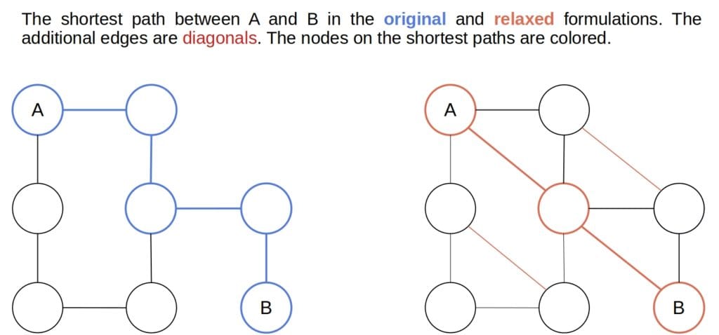
Since the relaxed problem has more edges in the state space, it’s easier to solve. The relaxed costs can serve as heuristics for the original problem.

6.2. Generating Heuristics from Subproblems

We can focus on a subproblem that’s easy to solve and use the cost of its solution as a heuristic function.

For instance, we can focus only on numbers 1-4 in the 8-puzzle game. Let’s use as a heuristic the length of the shortest sequence of moves that put only those four numbers in their goal positions.

Although the heuristic underestimates the cost of the optimal solution to the whole problem, it does hint at how much a state is far from the goal.

6.3. Learning Heuristics from Data

The third option is to learn heuristics from data. Let’s imagine a list of $(s, c)$ pairs, where $s$ is a state, and $c$ is the cost of the optimal path from $S$ to the goal. We can collect such a dataset by setting $s$ to be the start state and running an uninformed search strategy. To account for statistical variability, we randomly select a few problem instances and sample several states from their search spaces.

Afterward, we run an uninformed search on those inputs and collect the costs of the optimal solutions.

Once we create the dataset, we can treat it as a regression problem and apply a machine-learning algorithm to find a model that approximates the costs. Then, we use that model as our heuristic.

Sometimes, the state representation won’t be suitable for machine learning. That can happen if the states are structured objects that are hard to handle by traditional algorithms that expect vector data. To overcome this issue, we can represent the states by hand-selected or automatically engineered features.

For example, one feature $x_1$ in the puzzle problem can be the number of misplaced symbols-the very first heuristic we used. We can define another feature, $x_2$ , as the number of adjacent pairs that aren’t next to one another in the goal state. Then, we learn a mapping from $[x_1, x_2]$ to $c$ and use it as a heuristic.

7. Summary

Finally, this is the summary of informed vs. uninformed search strategies:

Uninformed Strategies	Informed Strategies
Use only the problem definition	Use a heuristic as a source of extra knowledge
Usually slower than the informed searches	Fast if the heuristic is efficient
All the computing happens inside the algorithm	Heuristics incur computational overhead
Require only the problem definition	Time has to be spent designing a quality heuristic

8. Conclusion

In this article, we talked about uninformed and informed search strategies. Uninformed algorithms use only the problem definition, whereas the informed strategies can also use additional knowledge available through a heuristic that estimates the cost of the optimal path to the goal state.

If the heuristic estimates are easy to compute, the informed search algorithms will be faster than the uninformed. That’s because the heuristic allows them to focus on the promising parts of the search tree. However, an efficient heuristic isn’t easy to formulate.

Learn Java Collections

Learn Spring

Learn Maven

View All Courses

Core Concepts

Operating Systems

Neural Networks

Graph Theory

Latex

Full Archive

About Baeldung