

Yes, we're now running our only Summer Sale. All Courses are 30% off until 20th July, 2026:
Introduction to Depth First Search Algorithm (DFS)
Last updated: March 24, 2023
Learn in
Learn through the super-clean Baeldung Pro experience:
>> Membership and Baeldung Pro.
No ads, dark-mode and 6 months free of IntelliJ Idea Ultimate to start with.
1. Overview
In graph theory, one of the main traversal algorithms is DFS (Depth First Search). In this tutorial, we’ll introduce this algorithm and focus on implementing it in both the recursive and non-recursive ways.
First of all, we’ll explain how does the DFS algorithm work and see how does the recursive version look like. Also, we’ll provide an example to see how does the algorithm traverse over a given graph.
Next, we’ll explain the idea behind the non-recursive version, present its implementation, and provide an example to show how both versions handle the example graph.
Finally, we’ll compare both the recursive and non-recursive versions and show when to use each one.
2. Definitions
Let’s start with defining the DFS algorithm in general, and provide an example to see how the algorithm works.
2.1. General Concept
The DFS algorithm starts from a starting node  . In each step, the algorithm picks one of the non-visited nodes among the adjacents of and performs a recursive call starting from that node. When all the neighbors of a node are visited, then the algorithm ends for the node and returns to check the neighbors of the node that initiated the call to node .
Unlike the BFS algorithm, DFS doesn’t visit nodes on a level-by-level basis. Instead, it keeps going deep as much as possible. Once the algorithm reaches an end, it tries to go deeper from other adjacents of the last visited node. Therefore, the name depth-first search comes from the fact that the algorithm tries to go deeper into the graph in each step.
For simplicity, we’ll assume that the graph is represented in the adjacency list data structure. All the discussed algorithms can be easily modified to be applied in the case of other data structures.
2.2. Example
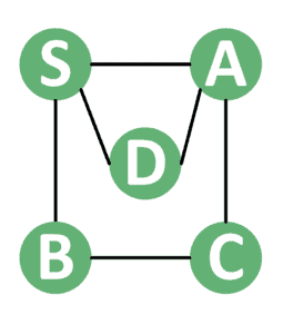
Consider the following graph example:

Suppose we were to start the DFS operation from node  . Let’s assume that all the neighboring nodes inside the adjacency list are ordered in the increasing order alphabetically. We’ll perform the following operations:
- Starting from , we have two neighbors,
 , and
, and  . Hence, we continue from .
 - Since only has one unvisited adjacent
 , we continue from that one.
 - The node has two unvisited neighbors
 and
and  . Hence, we continue from the node .
 - has only one unvisited neighbor that is . So, we move to .
- Similarly, has only one unvisited adjacent, which is
 . Therefore, the next node should be . Note that has also and as adjacents. But, these nodes are already visited.
 - has only that is unvisited. Thus, we move to .
- Finally, the node doesn’t have any unvisited neighbors. The algorithm will retract to , , , , , and then . These nodes won’t have any unvisited adjacents. So, the algorithm simply ends.
As a result, the final order of the visited nodes is { }.
}.
3. Recursive DFS
Let’s introduce the recursive version of the DFS algorithm. Take a look at the implementation:
algorithm RecursiveDFS(G, root):
    // INPUT
    //     G = the graph stored in the adjacency list
    //     root = the starting node
    // OUTPUT
    //     prints all nodes in the graph in the DFS order

    visited <- initialize all nodes as false
    DFS(root)

function DFS(u):
    if visited[u] = true:
        return
    print(u)
    visited[u] <- true
    for each v in G[u].neighbors():
        DFS(v)
First of all, we define the  array that will be initialized with
  values. The use of the
  array is to determine which nodes have been visited to prevent the algorithm from visiting the same node more than once.
Once the array is ready, we call the  function.
The function starts by checking whether the node is visited or not. If so, it just returns without performing any more actions.
However, if the node  isn’t visited, then the function prints it. Also, the function marks the node as visited to prevent it from being revisited in later steps.
Since the node was processed, we can iterate over its neighbors. For each one, we call the function recursively.
The complexity of the recursive version is  , where
  is the number of nodes, and is the number of edges inside the graph.
The reason behind the complexity is that we visit each node only once by the function. Also, for each node, we iterate over its neighbors only once. So, we’ll explore each edge inside the graph twice. Suppose the edge is between and  , then for the first time, we explore as the adjacent of , while in the second time, we discover as the adjacent of .
Therefore, in total, the inner  loop gets executed
  times.
Now that we have a good understanding of the recursive DFS version, we can update it to become iterative (non-recursive).
4. Iterative DFS
Let’s start by analyzing the recursive DFS version. From that, we can build the iterative approach step by step.
4.1. Analyzing the Recursive Approach
After reading the recursive DFS pseudocode, we can come to the following notes:
- For each node , the DFS function explores its neighboring nodes one by one. However, the function only performs a recursive call to the unvisited ones.
- When exploring the neighboring nodes, the next node that the DFS function will explore is the first unvisited node inside the adjacency list. This order must be respected.
- Once the DFS function finishes visiting the entire subgraph connected to a node, it terminates and returns to the previous node (the one that performed the recursive call on node ).
- How that works is that the program pushes the current parameters and variables of the function into a stack. Once the recursive call is finished, the program retrieves these variables from the stack and continues the execution. Hence, we need to use a manual stack to update the recursive DFS into the iterative version.
Let’s use the above notes to create the iterative version.
4.2. Theoretical Idea
What we need to do is to simulate the work of the program stack. First of all, let’s push the starting node into the stack. Then, we can perform multiple steps.
In each step, we’ll extract an element from the stack. This should be similar to starting a new recursive call for the DFS function. Once we pop a node from the stack, we can iterate over its neighbors.
To visit the adjacents of the extracted node, we need to push them into the stack as well. However, if we pushed the nodes into the stack and then extracted the next one, we’d get the last neighbor (because the stack serves as First-In-First-Out).
So, we need to add the nodes into the stack in the reversed order of their appearance inside the adjacency list. Note that this step is only mandatory if we need to follow the same order of the recursive version. If we don’t care about the order of the nodes inside the adjacency list, then we can simply add them to the stack in any order as well.
After that, we’ll extract a node from the stack, visit it and iterate over its neighbors. This process should continue until the stack becomes empty.
After listing the main ideas of the algorithm, we can organize a neat iterative implementation.
4.3. Implementation
Let’s take a look at the implementation of the iterative DFS.
algorithm IterativeDFS(G, root):
    // INPUT
    //     G = the graph stored in an adjacency list
    //     root = the starting node
    // OUTPUT
    //     prints all nodes in the graph in DFS order

    visited <- initialize all nodes as false
    stack <- create an empty stack
    stack.push(root)
    while stack is not empty:
        u <- stack.pop()
        if visited[u] = true:
            continue
        print(u)
        visited[u] <- true
        for each v in G[u]:
            if visited[v] = false:
                stack.push(v)
Similarly to the recursive version, we’ll initialize an array with values that will indicate whether we’ve visited each node so far or not. However, in the iterative version, we also initialize an empty stack that will simulate the program stack in the recursive version.
Next, we push the starting node into the stack. After that, we’ll perform multiple steps similar to the recursive version.
In each step, we extract a node from the stack, which simulates entering a new recursive DFS call. Then, we check whether we’ve already visited this node or not. If we did, then we continue without processing the node nor visiting its neighbors.
However, if the node isn’t visited, we print its value (indicating that we processed the node) and mark it as visited. Also, we iterate over all its adjacents and push them to the stack. Pushing the adjacents into the stack simulates performing a recursive call for each of them.
Nevertheless, in the iterative version, we must iterate over the neighbors in the reverse order. Therefore, we assume that ![G[u]](/wp-content/ql-cache/quicklatex.com-8a3d18e7690d093b959e3118c51710db_l3.svg "Rendered by QuickLaTeX.com") returns the adjacents of in the reversed order.
returns the adjacents of in the reversed order.
Also, instead of pushing all the neighbors into the stack, we’ll only push the non-visited ones. This step is unnecessary, but it allows us to reduce the number of nodes inside the stack, without affecting the results.
Since the steps of the iterative approach are identical to the recursive one, the complexity is , where is the number of nodes and is the number of edges inside the graph.
5. Example
Consider the following graph example:
Let’s see how does the recursive and non-recursive DFS versions print the nodes of this graph.
In the case of the recursive DFS, we show the first three steps in the example below:
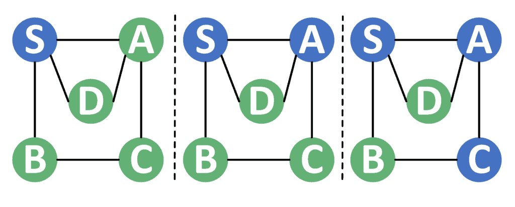
Note that the nodes whose recursive call didn’t end yet are marked with a blue color.
First of all, we start at the node . We explore its neighbors and therefore move to the node in the second step. After exploring the neighbors of the node , we continue to the node .
Now let’s see how the next three steps look like:
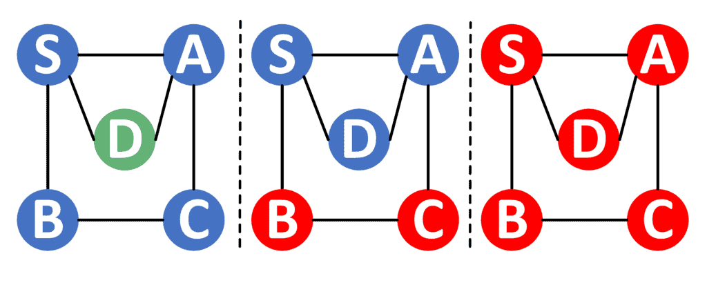
In this example, we have some nodes whose recursive function is finished. These nodes are marked with a red color.
From node we explore its neighbor and move to it.
Now, things get tricky. We notice that doesn’t have any non-visited neighbors. Therefore, we finish the recursive call on node and return to node .
However, the node doesn’t have any non-visited adjacents as well. Hence, we finish its recursive call too, and return to node .
We notice that node has a non-visited neighbor that is node . Thus, it performs a recursive call starting from node . However, node doesn’t seem to have any non-visited nodes. So, the function returns to node .
Since we finished visiting all the adjacents of node , the function returns to node . We notice that the node doesn’t have any more unvisited nodes. Hence, the function stops.
As a result, we notice that the visited nodes in order are { }.
}.
Now, let’s check how will the iterative approach handle the graph example.
5.1. Iterative DFS
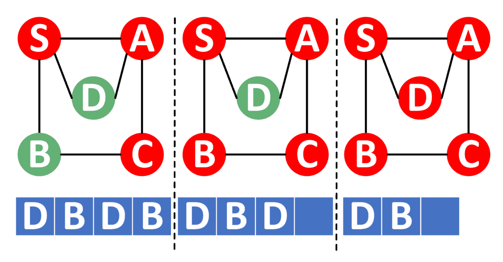
Consider the first three steps in case of the iterative DFS:
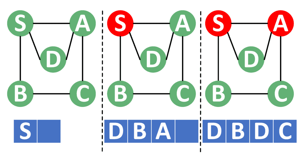
In the iterative DFS, we use a manual stack to simulate the recursion. The stack is marked with a blue color. Also, all the visited nodes so far are marked with a red color.
In the beginning, we add the node to the stack in the first step. Once we pop the nodes from the stack, it becomes visited. Therefore, we marked it with a red color. Since we visited node , we add all its neighbors into the stack in the reversed order.
Next, we pop from the stack and push all its unvisited neighbors and . In this case, we add node again to the stack. This is completely fine, because node is a neighbor to both and , and it’s still unvisited.
Let’s take a look at the next three steps of the iterative approach:
We pop node from the stack, mark it as visited, and push its adjacent .
The next step is to extract and mark as visited. However, in this case, node doesn’t have any unvisited neighbors. So, we don’t push anything into the stack in this case.
The next node we pop is node . Similarly, we’ve already visited all its neighbors, so we don’t push anything in its place.
After we visited all nodes, we still have nodes and inside the stack. So, we pop these nodes and continue because we’ve already visited both of them.
Note that we got a similar visiting order to the recursive approach. The order of the visiting is also {}.
Both the recursive and iterative approaches have the same complexity. Therefore, it’s usually easier to just use the recursive approach as it’s simpler to implement.
However, in rare cases, when the stack of the program has a small size, we might need to use the iterative approach. The reason is that the program allocates the manual stack inside the heap space, which is usually larger than the stack space.
6. Conclusion
In this tutorial, we introduced the depth-first search algorithm. First of all, we explained how the algorithm generally works and presented the implementation of the recursive version.
Next, we showed how to mock the recursive approach to implementing it iteratively.
After that, we provided a step-by-step example of both approaches and compared the results.
Finally, we summarized with a quick comparison that showed us when to use each approach.