Iterative Deepening vs. Depth-First Search | Baeldung on Computer Science

1. Introduction

In this tutorial, we’ll talk about two search algorithms: Depth-First Search and Iterative Deepening. Both algorithms search graphs and have numerous applications. However, there are significant differences between them.

2. Graph Search

In general, we have a graph with a possibly infinite set of nodes and a set of edges connecting them. Our goal is to find the shortest path between a start node $\boldsymbol{s}$ and a target node $\boldsymbol{t}$ .

A few variations of the problem are possible. In this article, we’ll assume that the edges are directed and have no weights, so the length of a path is precisely the number of edges it contains. For the alternative with weights, we use other algorithms. Because we’ll work with directed edges, we’ll say that the neighbors of a node are its children to emphasize the asymmetric nature of their relationship.

We’ll assume the graphs are implicit. That means that we have a function that receives a node at the input and returns its children. We lose no generality this way since the explicit graphs have a trivial implicit formulation. The same goes for the target node: we’ll assume there’s a function that can test if a node qualifies as a target. This way, we cover the cases when there’s more than one target node in the graph.

2.1. Example

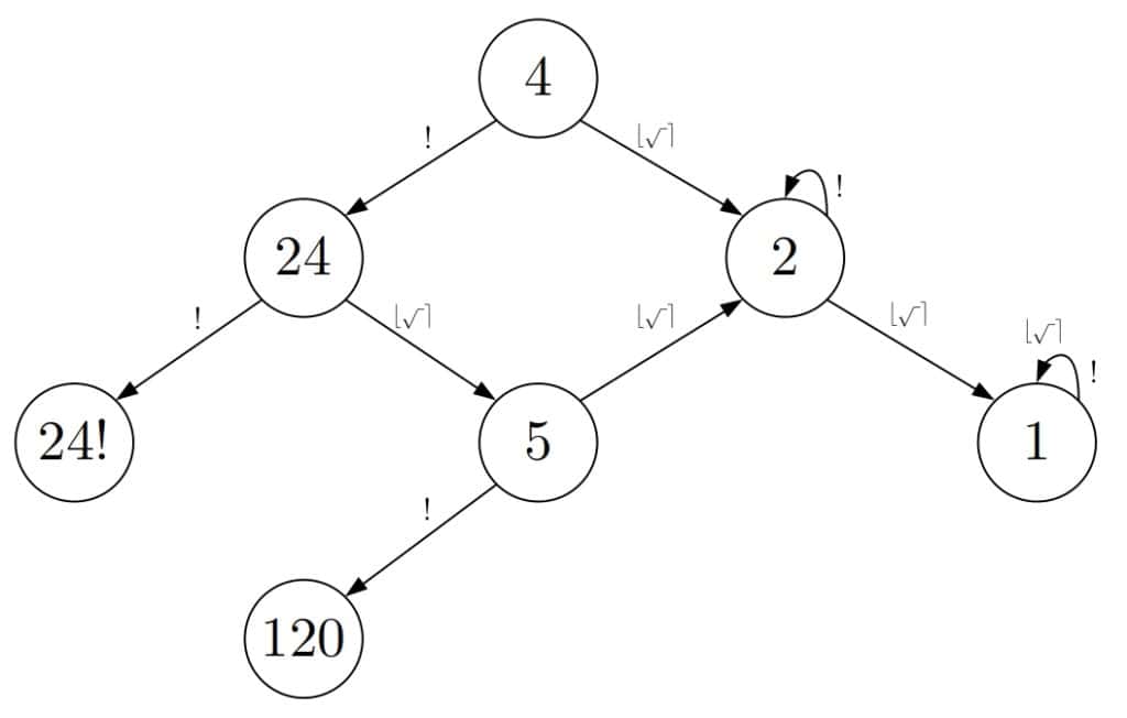
We’ll base our working example on the Knuth’s conjecture about positive integers. Knuth conjectured in 1964 that every positive integer could be obtained by applying a finite sequence of the square root, floor, and factorial operations starting from number 4. For instance:

(1) $\begin{equation*} 5 = \left\lfloor \sqrt{\sqrt{\sqrt{\sqrt{\sqrt{(4!)!}}}}} \right\rfloor \end{equation*}$

To make the example easier to present, we’ll use rounding to the nearest integer ( $\lfloor \cdot \rceil$ ) instead of flooring.

In the corresponding graph, the nodes are positive real numbers. The start node is number 4. There’s a directed edge between nodes $u$ and $v$ if $v=\sqrt{u}$ , $v=u!$ , or $v=\lfloor u \rceil$ . Given any number $r > 0$ , we want to find the shortest sequence of the operations that reach it starting from 4. That sequence corresponds to the shortest path between 4 and $r$ in the implicit graph. Then, the target test function is:

$target(x) = \begin{cases} true ,& x = r\\ false,& x \neq r \end{cases}$

Let’s note that we should round only non-integers and that only square root can produce them. Also, we should apply factorial only to integer numbers. With that in mind, let’s take a look at a small portion of the search graph:

2. Depth-First Search

Depth-First Search (DFS) begins the search at the start node $s$ . It first tests $s$ to see if it’s the target. If not, then DFS identifies and tests its children as the next step. This step is called expansion. We call a node expanded (or explored) if DFS has identified its children. Those children we call visited. If no child passes the test, then DFS picks the most recently visited but unexpanded child $v$ and repeats the steps.

It goes deeper and deeper in the graph until it finds the target or has to backtrack to a node $\boldsymbol{w}$ because the current node has no children. After backtracking, DFS expands the second child of $w$ and continues the search until it reaches a target node or explores all the nodes.

2.1. Example

Let’s see how DFS would handle our example with numbers:

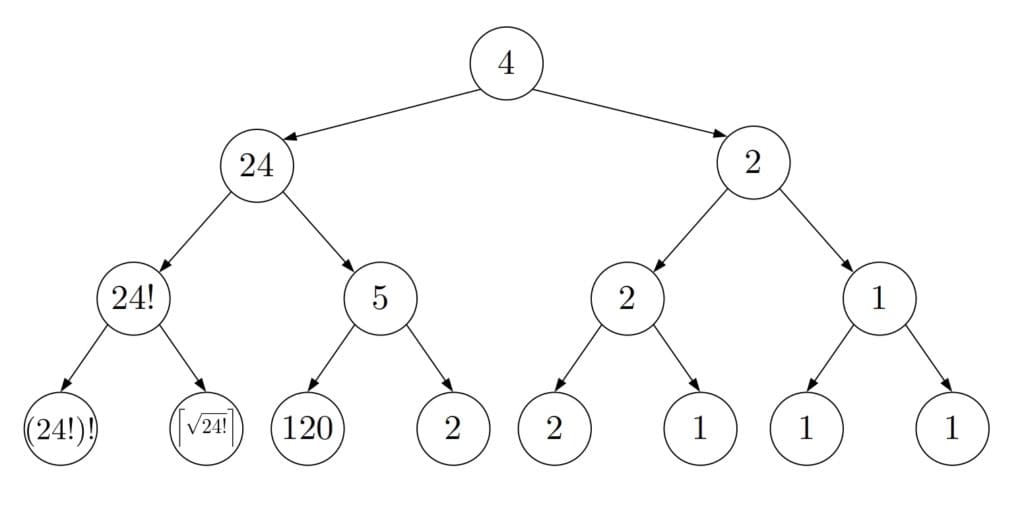
We see that DFS creates a tree whose root is the start node. The search would continue beyond the third level, and the tree would grow exponentially until the search stopped.

2.2. The Algorithm

We can implement DFS with or without recursion. Here, we’ll work with the recursive version:

This version of DFS is known as the tree-search DFS (TSDFS) because it terminates if the graph is a (finite) tree. If the search graph isn’t a tree, then TSDFS can get stuck in a loop. To avoid infinite loops, DFS should keep track of the nodes it expanded. That way, it doesn’t explore any node more than once, so it can’t get stuck in a loop. We call that version of DFS a graph-search DFS (GSDFS) since it can handle graphs in general, not just trees.

3. Iterative Deepening

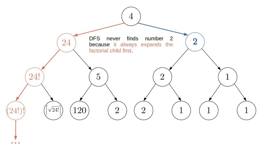
DFS has two shortcomings:

It may miss the optimal path. Depending on the order in which $children$ returns the children of a node, DFS may expand more nodes than necessary:

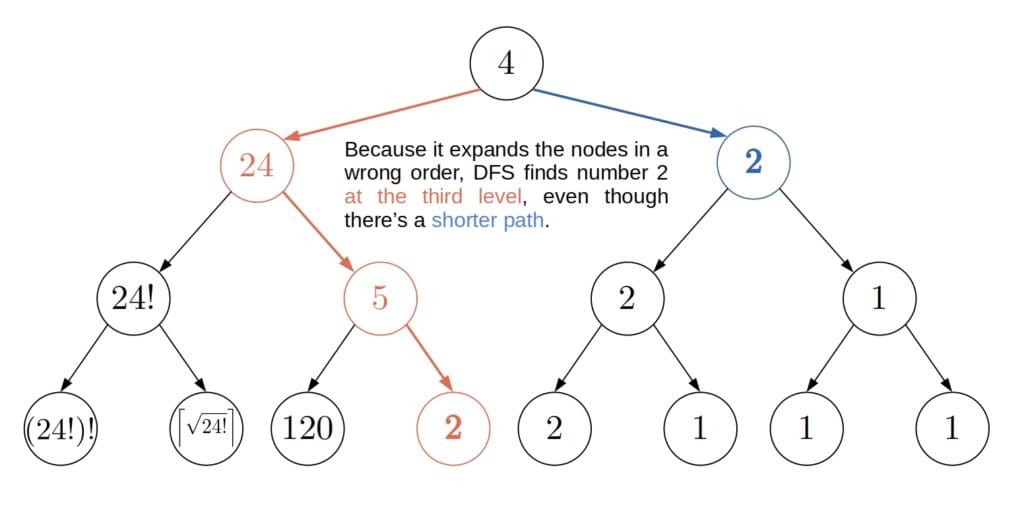
Also, DFS may never end! It may get stuck at expanding the nodes that can’t lead to a target node even if we use the graph-search version of the algorithm:

Iterative Deepening (ID) solves both problems. It relies on depth-limited DFS.

3.1. Depth-Limited DFS

Depth-limited DFS (DLDFS) runs just as DFS but with an additional stopping criterion. Namely, it explores only the nodes whose distances to the start node, i.e., their depths in the search tree, are at most $\boldsymbol{\ell} \boldsymbol{\geq} \boldsymbol{1}$ . With a finite $\ell$ , DLDFS will terminate. It’s up to us to choose a suitable value of $\ell$ in advance.

If we set $\ell=d$ , where $d$ is the depth of the target node closest to the start, then DLDFS will find the shortest path. Why? Because it will explore all the nodes whose depth is at most $d$ and there aren’t any target nodes at a depth smaller than $d$ . However, if $\ell < d$ , then DLDFS will not be able to reach it. Furthermore, if $\ell > d$ , then DLDFS may find a suboptimal path to a target node. But, if no target node is reachable from the start vertex, then DLDFS will always fail, no matter the limit depth $\ell$ .

So, there are three ways in which DLDFS can terminate:

it finds a path (the shortest or suboptimal)
it fails to find a path to a target node because the limit depth is too shallow
it doesn’t find a path because there is none

3.2. Pseudocode

The pseudocode of DLDFS is similar to that of DFS:

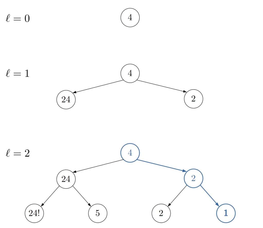
We don’t have to worry about expanding the same node more than once. The depth limit makes sure that exploration of all paths eventually stops. For instance, with $\ell=3$ , DLDFS would would stop right after the third level.

3.3. Deepening

Deepening sorts out the problems of DLDFS and DFS. The idea is to try out incremental values $\boldsymbol{0},\boldsymbol{1},\boldsymbol{2},\ldots$ as the depth limit $\boldsymbol{\ell}$ until DLDFS finds a target node. Since we increment the limit depth by $1$ , we know that the first path DLDFS finds is the shortest among all that end in a target node: had it been otherwise, DLDFS would’ve found another path at a shallower depth.

This is the pseudocode of iterative deepening:

3.4. Example

Let’s say that we search for the number 1. ID starts with $\ell=0$ and inspects the start node only. Then, it increments $\ell$ and restarts the search, stopping after the first level. Finally, with $\ell=2$ , ID finds number 1:

Without deepening, DFS could miss the shortest path or never end.

3.5. Comparison to Breadth-First Search

Breadth-First Search (BFS) explores the nodes one level at a time. It first expands the start node’s children. Only when it processes all of them does BFS expands their children. ID is similar in the sense that it explores the nodes at depth $\ell$ only after it’s expanded all the nodes at the depths $1,2,\ldots,\ell-1$ . But, the difference is that ID successively processes the nodes at incremental depths, whereas BFS conducts the search level by level. Also, BFS visits each node once, whereas ID visits some nodes multiple times since it restarts DLDFS.

3.6. Couldn’t We Randomize DFS?

We may think that there’s a simpler solution. Instead of deepening, couldn’t we randomize the order in which function $children$ returns the nodes? The answer is that, even though we’d make the worst-case scenario and infinite loops less likely that way, we still wouldn’t rule them out. There would still be a small probability that DFS runs forever or returns a suboptimal path.

4. Comparison

We’ll compare DFS to ID in terms of

completeness
optimality
time complexity
space complexity

Completeness refers to the existence of guarantees that the algorithm at hand returns either a path to a target node or a message that it couldn’t reach such a node. Optimality means that the algorithm finds the shortest path to a target node, not just any path to it.

When it comes to complexity analysis, let’s set up the notation first. We’ll denote as $d$ the length of the shortest path from the start node to a target node (which corresponds to the node’s depth in the search tree), as $b$ the maximal number of children a node has in the graph, and as $m$ the length of the longest path between any two nodes in the graph.

4.1. Completeness and Optimality

DFS isn’t complete. The tree-search version can get stuck in loops, while the graph-search variant may run forever in infinite graphs. On the other hand, ID is always complete if no node has an infinite number of children. If that’s the case with at least one node at a depth lower than $d$ , and no target node is among its successors, then ID will be expanding the node’s children forever.

Regarding optimality, ID will detect the shortest path to a target node or conclude that no target node is reachable from the start vertex if the completeness condition holds. In contrast, both TSDFS and GSDFS may find a suboptimal path. The order in which $children$ returns the children of a node determines if the found path will be optimal.

4.2. Time Complexity

In the worst case, GSDFS explores the whole graph by processing each node once and each edge twice, so its complexity is $O(n_V+n_E)$ , where $n_V$ is the number of nodes and $n_E$ is the number of edges in the graph. Because it can expand a node more than once, TSDFS’s complexity is not bounded by the size of the graph. Instead, TSDFS can generate a search tree with $\boldsymbol{O(b^m)}$ leaves. So, its complexity is:

(2) $\begin{equation*} 1+b+b^2+\ldots+b^{m} \in O(b^{m}) \end{equation*}$

which can also serve as an upper bound of the graph’s size. It’s also the upper bound of the complexity of GSDFS in the cases we don’t know $n_V$ and $n_E$ but know or can guess $b$ and $m$ .

The complexity of ID is as follows. The algorithm explores the start node $d+1$ times, its children $d$ times, and so on. It explores the nodes at the depth $d$ in the search tree only once and doesn’t visit any other node because the shortest path is at depth $d$ . There are no more than $b$ children of the start node, no more than $b^2$ nodes at depth 2, and so on. Therefore, ID explores this many nodes at most:

(3) $\begin{equation*} (d+1) + db + (d-1)b^2+\ldots+b^d \in O(b^d) \end{equation*}$

so its time complexity is $\boldsymbol{O(b^d)}$ . Since $\boldsymbol{d} \boldsymbol{\leq} \boldsymbol{m}$ , we conclude that ID beats DFS by this criterion too.

4.3. Why Isn’t Iterative Deepening Slower?

The lower complexity of ID in comparison to DFS may come as somewhat counter-intuitive. After all, GSDFS expands each node once, and we can modify TSDFS to memorize the current path to avoid loops, whereas ID for each $\ell$ revisits all the nodes at depths $1, 2, \ldots, \ell-1$ .

Even though it might seem that ID does an order of magnitude more work, it’s not the case. If all the nodes have approximately the same number of children, then most of the nodes will belong to the bottom levels of the search tree rooted at the start node. Hence, the nodes at the upper levels of the tree account for a relatively small share of all the nodes, so revisiting them several times doesn’t add too much overhead. For instance, if all the nodes have 5 children, then the leaves of the search tree make up for approximately 80% of the tree. The second-to-last level accounts for another 16%. So, only 4% of the tree is processed more than two times.

4.4. Space Complexity

GSDFS has an $\boldsymbol{O(n_V)}$ worst-case space complexity since it memorizes all the nodes it expands and explores the whole graph in the worst-case scenario. In contrast, TSDFS needs to keep track only of the visited but unexpanded children of the nodes along the current path. So, its space complexity is $\boldsymbol{O(bm)}$ since $m$ is the upper limit of the path’s length and no node in it has more than $b$ children.

Our ID uses depth-limited tree-search DFS, so its space complexity is $\boldsymbol{O(bd)}$ because DLDFS with depth limit $\ell$ has an $O(b\ell)$ space complexity.

4.5. Summary

So, ID is complete even in the cases DFS is not, returns the shortest path if one exists, has a better time complexity, and requires less memory:

5. Conclusion

In this article, we talked about Depth-First Search and Iterative Deepening. We explained why the latter has lower space and time complexities. Also, we showed why it’s complete and comes with guarantees to find the shortest path if one exists. However, we assumed that the edges in the search graph were without weights. If the assumption doesn’t hold, then we should use other algorithms.

Full Archive

About Baeldung

Core Concepts

Operating Systems

Artificial Intelligence

Graph Theory

Latex

1. Introduction

2. Graph Search

2.1. Example

2. Depth-First Search

2.1. Example

2.2. The Algorithm

3. Iterative Deepening

3.1. Depth-Limited DFS

3.2. Pseudocode

3.3. Deepening

3.4. Example

3.5. Comparison to Breadth-First Search

3.6. Couldn’t We Randomize DFS?

4. Comparison

4.1. Completeness and Optimality

4.2. Time Complexity

4.3. Why Isn’t Iterative Deepening Slower?

4.4. Space Complexity

4.5. Summary

5. Conclusion