

Yes, we're now running our only Summer Sale. All Courses are 30% off until 20th July, 2026:
Difference Between BFS and Dijkstra’s Algorithms
Last updated: March 18, 2024
Learn through the super-clean Baeldung Pro experience:
>> Membership and Baeldung Pro.
No ads, dark-mode and 6 months free of IntelliJ Idea Ultimate to start with.
1. Overview
In graph theory, SSSP (Single Source Shortest Path) algorithms solve the problem of finding the shortest path from a starting node (source), to all other nodes inside the graph. The main algorithms that fall under this definition are Breadth-First Search (BFS) and Dijkstra‘s algorithms.
In this tutorial, we will present a general explanation of both algorithms. Also, we will show the differences between them and when to use each one.
2. General Algorithm
Both algorithms have the same general idea. We start from the source node and explore the graph, node by node. In each step, we always go to the node that is closest to the source node.
Let’s see a flow chart that better explains the general algorithm:
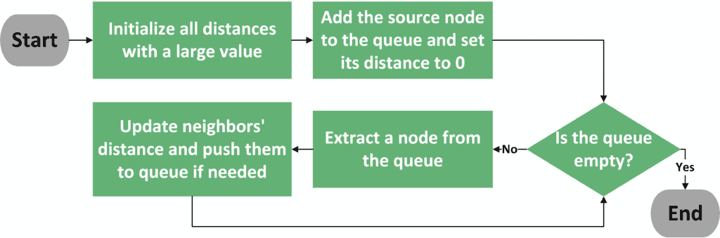
As you can see, the first two steps are to initialize the distances with a large value and to add the source node to the queue. Next, we perform iterations until the queue becomes empty. In each iteration, we extract a node from the queue that has the shortest distance from the source node.
After that, we visit all the neighbors of the extracted node and check the new distance we were able to achieve. If the new distance is better than the old one, we update the distance of this node and push it to the queue. Finally, the algorithm moves to perform one more iteration until the queue becomes empty.
After the algorithm ends, we’ll have the shortest paths from the source node to all other nodes in the graph.
However, since graphs are either weighted or unweighted, we can’t use the exact same algorithm for both cases. Therefore, we have two algorithms. BFS calculates the shortest paths in unweighted graphs. On the other hand, Dijkstra’s algorithm calculates the same thing in weighted graphs.
3. BFS Algorithm
When dealing with unweighted graphs, we always care about reducing the number of visited edges. Therefore, we are sure that all the direct neighbors of the source node have a distance equal to one. The next thing that we can be sure about is that all the second neighbors of the source node have a distance equal to two, and so on.
This idea continues to be valid until we cover all the nodes of the graph. The only exception is if we reached a node that has been visited before. In this case, we should ignore it. The reason is that we must have reached it with a shorter path before.
It’s worth noting that in weighted graphs, where all edges have the same weight, the BFS algorithm calculates the shortest paths correctly. The reason is that it cares about reducing the number of visited edges, which is true in case of equal weights for all edges.
Let’s think about the updates that need to be done to our general algorithm. The main approach we follow is to always start from a node we reached earlier. This looks similar to the concept of FIFO (First In First Out) that we can find in a simple queue. Therefore, we use a simple queue with BFS. We can see that there are no more updates that we should do to our general algorithm.
Since we’re using an ordinary queue, we have an  time complexity for push and pop operations. Therefore, the total time complexity is
  , where
  is the number of vertices and
  is the number of edges in the graph.
4. Dijkstra’s Algorithm
When it comes to weighted graphs, it’s not necessary that neighboring nodes always have the shortest path. However, the neighbor with the shortest edge can’t be reached by any shorter path. The reason is that all other edges have larger weights, so going through them alone would increase the distance.
Dijkstra’s algorithm uses this idea to come up with a greedy approach. In each step, we choose the node with the shortest path. We fix this cost and add this node’s neighbors to the queue. Therefore, the queue must be able to order the nodes inside it based on the smallest cost. We can consider using a priority queue to achieve this.
We still have one problem. In unweighted graphs, when we reached a node from a different path, we were sure that the first time should have the shortest path. In weighted graphs, that’s not always true. If we reached the node with a shorter path, we must update its distance and add it to the queue. This means that the same node could be added multiple times.
Therefore, we must always compare the cost of the extracted node with its actual stored cost. If the extracted distance is larger than the stored one, it means this node was added in an early stage. Later, we must have found a shorter path and updated it. We have also added the node again to the queue, so this extraction can be ignored safely.
Since we’re visiting each nodes’ neighbors only once, we’re visiting edges only once as well. Also, we can use a priority queue that has a time complexity of  for push and pop operations. Therefore, the total time complexity is
  .
.
5. Example
Take a look at the following graph. It contains an example of applying the BFS algorithm to a simple, unweighted graph. The letter corresponds to the node index, while the number shows the stored distance after performing the BFS algorithm:
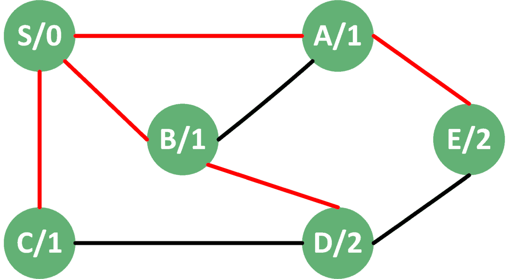
We can clearly see that the algorithm visits the nodes, level by level. First, all the neighbors  are visited on level 1. Next, all the second neighbors
  are visited on level 2, and so on. As a result, we’re able to calculate the shortest path to all nodes starting from the source node
  .
.
Now, let’s take a look at the result of applying Dijkstra’s algorithm to the weighted version of the same graph:
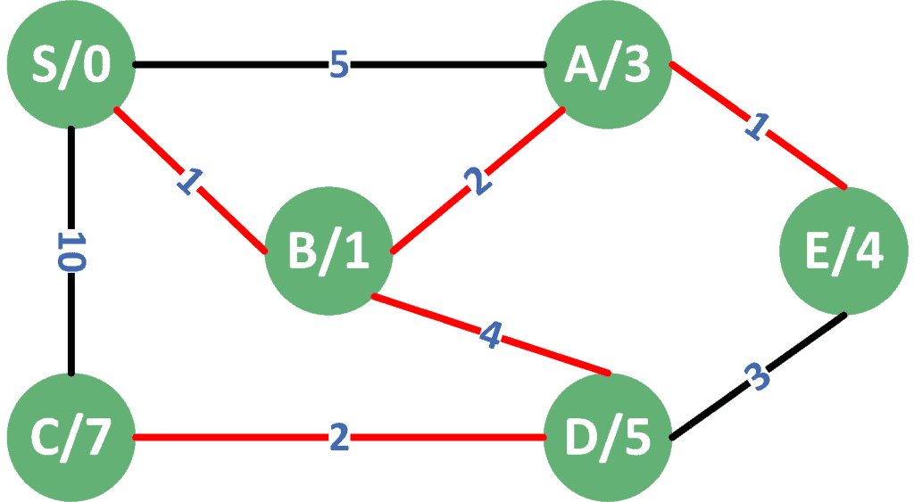
Although node  is one step away from the source , Dijkstra’s algorithm first explored node
  because the edge to has the lowest cost.
Next, from , it found a shorter path to node , which is the path that the algorithm stored.
We can also note that although it’s one step away from , we didn’t visit  directly. The reason is that the edge between and has a very large cost. Luckily, we were able to reach from a shorter path than the direct edge.
6. Comparison
The following table shows a summarized comparison between the two algorithms:
| BFS | Dijkstra | |
|---|---|---|
| Main Concept | Visit nodes level by level based on the closest to the source |
In each step, visit the node withthe lowest cost |
| Optimality | Gives an optimal solution for unweighted graphs orweighted ones with equal weights |
Gives an optimal solution for both weightedand unweighted graphs |
| Queue Type | Simple queue | Priority queue |
| Time Complexity | |
 |
7. Conclusion
In this tutorial, we presented the general algorithm for BFS and Dijkstra’s algorithms. Next, we explained the main similarities and differences between the two algorithms.
After that, we took a look at the result of applying both algorithms to unweighted and weighted versions of the same graph.
Finally, we gave a comparison between both algorithms.