

Yes, we're now running our only Summer Sale. All Courses are 30% off until 20th July, 2026:
Obtaining the Path in the Uniform Cost Search Algorithm
Last updated: March 18, 2024
Learn through the super-clean Baeldung Pro experience:
>> Membership and Baeldung Pro.
No ads, dark-mode and 6 months free of IntelliJ Idea Ultimate to start with.
1. Overview
In this tutorial, we’ll discuss the problem of obtaining the path in the uniform cost search algorithm.
First, we’ll define the problem and provide an example that explains it.
Then we’ll discuss two different approaches to solve this problem.
2. Defining the Problem
Suppose we have a graph,  , that contains
  nodes. In addition, we have
  edges that connect these nodes. Each of these edges has a weight associated with it, representing the cost to use this edge. We’re also given two numbers,
  and
and  , that represent the source node and the destination node, respectively.
Our task is to find the path from the source node to the destination using the uniform cost search algorithm. Let’s look at an example for better understanding.
Suppose we have the following graph and we’re given  and
and  :
:
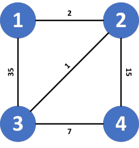
To go from node to node we have four possible paths:
 , with cost equal to
  .
. , with cost equal to
  .
. , with cost equal to
  .
. , with cost equal to
  .
.
When we apply the uniform cost search algorithm, we will get the minimal cost to go from the source node to the destination node . In this example, the cost will be equal to ; therefore, the path that the algorithm will detect between nodes  and
and  is
is  .
.
3. Naive Approach
3.1. Main Idea
The main idea here is to store all the nodes that are on the path from the source node to the destination. For every node, we’ll store two values:
 : which represents the cost of the path from the source node to the current one
 : which represents a list of nodes that lies on the path with the minimum cost from the source node to the current one
During uniform cost search, when we reach a child node with a smaller cost than the previous one, we’ll update the value for the child node to the new cost. In addition, we’ll change the value to be equal to the value of the  node after appending the child node to it.
In the end, the value of the node will have a list representing the path that goes from the source node to the destination with the minimum cost value. Also, the cost value of will be equal to the minimum cost to go from to .
3.2. Implementation
Let’s take a look at the implementation:
algorithm NaiveApproach(V, G, S, D):
    // INPUT
    //    V = Number of nodes in the graph
    //    G = The graph stored as an adjacency list
    //    S = The index of the source node
    //    D = The index of the destination node
    // OUTPUT
    //    Returns the path between S and D with minimum cost
    cost <- an array with all elements initialized to infinity
    path <- an empty set
    priorityQueue <- an empty queue
    priorityQueue.add(S)
    cost[S] <- 0
    path[S] <- [S]
    while not priorityQueue.empty():
        current <- priorityQueue.front()
        priorityQueue.pop()
        for child in G[current]:
            if cost[child] > cost[current] + weight(current, child):
                priorityQueue.add(child)
                cost[child] <- cost[current] + weight(current, child)
                path[child] <- path[current]
                path[child].append(child)
    return path[D]
Initially, we declare the and the arrays. The value for all nodes is infinity, except the source node, which is equal to  (the length of the path from a node to itself equals
  ). Furthermore, the value for all nodes is an empty list, except the source node, which is equal to a list containing the source node (a path from a node to itself contains just the node itself).
We also declare an empty priority queue to store the explored nodes sorted in the ascending order according to their cost value.
Next we perform multiple steps as long as the priority queue isn’t empty. In each step, we take the node positioned in the front of the queue and iterate over its children. For each child node, we check whether it has a value greater than the value of the node plus the weight of the edge that connects the node with the  node.
node.
If so, we add it to the priority queue, and we update its value to be equal to the of the current node plus the weight of the edge that connects it with the node. We also update its value to be equal to the value of the node, since the path that goes from the source to the child node passing through the node has a smaller cost. Then we append the node to its value.
Note that we need to copy the list using the deep copy technique. We want to take a copy of the list, including its element, and not just copy the reference to the list itself.
Finally, we return ![path[D]](/wp-content/ql-cache/quicklatex.com-6b81940a9faba4543df6b1ad9fb4dda4_l3.svg "Rendered by QuickLaTeX.com") , which stores a list of nodes that represent the smallest cost path that goes from the source to the destination .
, which stores a list of nodes that represent the smallest cost path that goes from the source to the destination .
3.3. Complexity
The time complexity here is a little different from the uniform cost search complexity. The uniform cost search algorithm has a complexity equal to  , where is the number of nodes and is the number of edges. However, since in this approach we store a list containing the path of each node, the complexity for this approach will be
  . This is because each list can have a size equal to in the worst case. Also, we might need to update each list times.
The space complexity is  in the worst-case scenario, since each time we store all the nodes from the source node to the current node.
4. Optimized Approach
4.1. Main Idea
We’ll apply the same concepts from the previous approach, but instead of storing all the nodes that lie on the path from the source node to the current node, we’ll just store the  node that comes before the node in the path. In the previous approach, the of each node was similar to its parent after appending the current node. Thus, we can only store the node instead of copying the complete list into the node.
After finishing the uniform cost search algorithm, we’ll append the destination node to the path and move to the node and add it to the beginning of the path. We’ll keep following the nodes until we reach the source node . At that point, we’ll have the path that goes from node to node .
4.2. Implementation
Let’s take a look at the implementation:
algorithm OptimizedApproach(V, G, S, D):
    // INPUT
    //    V = Number of nodes in the graph
    //    G = The graph stored as an adjacency list
    //    S = The index of the source node
    //    D = The index of the destination node
    // OUTPUT
    //    Returns the path from S to D with minimum cost using parent tracing
    cost <- an array with all elements initialized to infinity
    parent <- an array with all elements initialized to null
    priorityQueue <- {}
    priorityQueue.add(S)
    cost[S] <- 0
    while not priorityQueue.empty():
        current <- priorityQueue.front()
        priorityQueue.pop()
        for child in G[current]:
        if cost[child] > cost[current] + weight(current, child):
            priorityQueue.add(child)
            cost[child] <- cost[current] + weight(current, child)
            parent[child] <- current
    path <- []
    node <- D
    while node != null:
        path.add_front(node)
        node <- parent[node]
    return path
Initially, we declare the same array and priority queue from the previous approach. We also declare the array that will store the node that should come before the current node in the path.
Next we’ll perform the same steps from the previous approach; however, when we update the value of the node, we’ll update the value of the node to be equal to the node.
After finishing the uniform cost search, we declare the list that will store the source’s path to the destination. We also declare  , which is initially equal to the destination node. Then, while isn’t equal to
  , we add the to the beginning of the list and move to the of .
The reason we keep moving until we reach the value is that only the source doesn’t have a parent. Furthermore, we add the node to the beginning of the list because we’re moving from the last node in the path to the first node . Since we’re moving backward, we add the new node at the beginning of the list.
Finally, we return , which stores a list of nodes that represent the path that goes from the source node to the destination .
4.3. Complexity
The time complexity here is  , where is the number of nodes and is the number of edges. This is because we don’t copy the list anymore; instead, we only set the value.
The space complexity is  since we just store a single value for each node.
5. Conclusion
In this article, we presented the problem of obtaining the path in the uniform cost search algorithm. We explained the main ideas behind two different approaches to solving this problem and worked through their implementation.