Node Impurity in Decision Trees | Baeldung on Computer Science

1. Introduction

In this tutorial, we’ll talk about node impurity in decision trees. A decision tree is a greedy algorithm we use for supervised machine learning tasks such as classification and regression.

2. Splitting in Decision Trees

Firstly, the decision tree nodes are split based on all the variables. During the training phase, the data are passed from a root node to leaves for training. A decision tree uses different algorithms to decide whether to split a node into two or more sub-nodes. The algorithm chooses the partition maximizing the purity of the split (i.e., minimizing the impurity). Informally, impurity is a measure of homogeneity of the labels at the node at hand:

Very Impure, Less Impure, and Minimum Impurity Achieved at three nodes

There are different ways to define impurity. In classification tasks, we frequently use the Gini impurity index and Entropy.

3. Gini Impurity

Gini Index is related to the misclassification probability of a random sample.

Let’s assume that a dataset $T$ contains examples from $n$ classes. Its Gini Index, $gini(T)$ , is defined as:

(1) $\begin{equation*} gini(T) = 1 - \sum_{j=1}^{n} p_{j}^2 \end{equation*}$

where $p_j$ is the relative frequency of class $j$ in $T$ , i.e., the probability that a randomly selected object belongs to class $j$ .

As we can observe from the above equation, Gini Index may result in values inside the interval $[0, 0.5]$ . The minimum value of zero corresponds to a node containing the elements of the same class. In case this occurs, the node is called pure. The maximum value of 0.5 corresponds to the highest impurity of a node.

3.1. Example: Calculating Gini Impurity

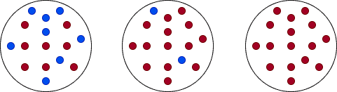
In this example, we’ll compute the Gini Indices for 3 different cases of a set with 4 balls of two different colors, red and blue:

4 red & 0 blue balls:
$gini = 1 - \left(P(ball = red)^2 + P(ball = blue)^2\right) = 1 - (1 + 0) = 0$
2 red & 2 blue balls:
$gini = 1 - \left(P(ball = red)^2 + P(ball = blue)^2\right) = 1 - \left(\left(\frac{1}{2}\right)^2 + \left(\frac{1}{2}\right)^2\right) = 0.5$
3 red & 1 blue balls:
$gini = 1 - \left(P(ball = red)^2 + P(ball = blue)^2\right) = 1 - \left(\left(\frac{3}{4}\right)^2 + \left(\frac{1}{4}\right)^2\right) = 0.375$

4. Entropy

Ιn statistics, entropy is a measure of information.

Let’s assume that a dataset $T$ associated with a node contains examples from $n$ classes. Then, its entropy is:

(2) $\begin{equation*} entropy(T) = - \sum_{j=1}^{n} p_j\cdot \log p_j \end{equation*}$

where $p_j$ is the relative frequency of class $j$ in $T$ . Entropy takes values from $[0, 1]$ . As is the case with the Gini index, a node is pure when $entropy(T)$ takes its minimum value, zero, and impure when it takes its highest value, 1.

4.1. Example: Calculating Entropy

Let’s compute the entropies for the same examples as above:

4 red & 0 blue balls:
$entropy = P(ball = red) \cdot log_2 P(ball = red) + P(ball = blue) \cdot log_2 P(ball = blue) = \frac{4}{4} \cdot log_2\frac{4}{4} - \frac{0}{4} \cdot log_2\frac{0}{4} = 0$
2 red & 2 blue balls:
$entropy = P(ball = red) \cdot log_2 P(ball = red) + P(ball = blue) \cdot log_2 P(ball = blue) = \frac{2}{4} \cdot log_2\frac{2}{4} - \frac{2}{4} \cdot log_2\frac{2}{4} = 1$
3 red & 1 blue balls:
$entropy = P(ball = red) \cdot log_2 P(ball = red) + P(ball = blue) \cdot log_2 P(ball = blue) = \frac{3}{4} \cdot log_2\frac{3}{4} - \frac{1}{4} \cdot log_2\frac{1}{4} = 0.811$

5. Splitting the Data

The quality of splitting data is very important during the training phase. When splitting, we choose to partition the data by the attribute that results in the smallest impurity of the new nodes.

We’ll show how to split the data using entropy and the Gini index.

5.1. Information Gain

The information gain is the difference between a parent node’s entropy and the weighted sum of its child node entropies.

Let’s assume a dataset $T$ with $N$ objects is partitioned into two datasets: $T_1$ and $T_2$ of sizes $N_1$ and $N_2$ . Then, the split’s Information Gain ( $Gain_{split}$ ) is:

(3) $\begin{equation*} {Gain_{split}(T) = entropy(T) - \frac{N_1}{N}\cdot entropy(T_1) - \frac{N_2}{N} \cdot Entropy(T_2) } \end{equation*}$

In general, if splitting $T$ into $m$ subsets $T_1, T_2, \ldots, T_m$ with $N_1, N_2, \ldots, N_m$ objects, respectively, the split’s Information Gain ( $Gain_{split}$ ) is:

(4) $\begin{equation*} {Gain_{split}(T) = entropy(T) - \frac{N_1}{N}\cdot entropy(T_1) - \frac{N_2}{N} \cdot entropy(T_2)- \ldots - \frac{N_m}{N}\cdot entropy(T_m) } \end{equation*}$

5.2. Example: Splitting by Information Gain

Let’s consider dataset $T$ , which shows if we’re going to play tennis or not based on the weather:

It contains 9 positive outcomes (Yes) and 5 negatives (No). So, the starting structure is $S=[9+, 5-]$ . We want to determine the attribute that offers the highest Information Gain.

Let’s see what happens if we split by Outcome. Outlook has three different values: Sunny, Overcast, and Rain. As we see, the possible splits are $[2+, 3-], [4+, 0-]$ and $[3+, 2-]$ ( $E$ and $S$ stand for entropy and split):

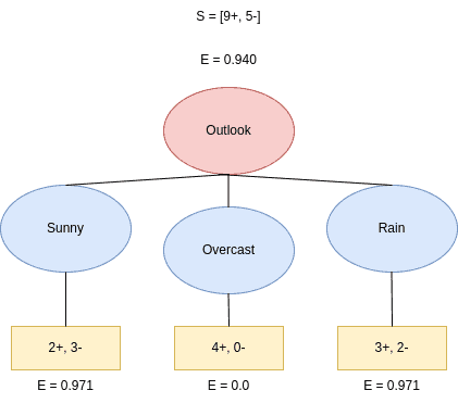
Decision Tree based on the <em>Outlook</em> feature

Firstly, we calculate the entropies. They are: $E(Sunny) = 0.971 , E(Overcast) = 0$ and $E(Rain) = 0.971$ . Therefore, the Information Gain based on the Outlook, $Gain(S, Outlook)$ , is:

(5) $\begin{equation*} {Gain(S, Outlook) = 0.940 - \frac{5}{14}\cdot0.971 -\frac{4}{14} \cdot0.0 -\frac{5}{14} \cdot0.971 = 0.247 } \end{equation*}$

Next, we split the tree based on the Wind feature. It can take two values: Weak and Strong, with the possible splits $[6+, 2-]$ and $[3+, 3-]$ :

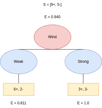
The corresponding entropies are: $E(Weak) = 0.811$ and $E(Strong) = 1.0$ . Therefore, $Gain(S, Wind)$ is:

(6) $\begin{equation*} {Gain(S, Wind) = 0.940 - \frac{8}{14}\cdot0.811 -\frac{6}{14} \cdot1.0 = 0.048 } \end{equation*}$

Following this idea, we calculate the gains for Humidity and Temperature as well.

(7) $\begin{equation*} {Gain(S, Humidity) = 0.151 } \end{equation*}$

(8) $\begin{equation*} {Gain(S, Temperature) = 0.029 } \end{equation*}$

We see that the feature with the maximum Information Gain is Outlook. Thus, we conclude that Outlook is the best attribute to split the data at the tree’s root.

5.3. Example: Splitting by Gini Index

We can split the data by the Gini Index too. Let’s compute the required probabilities:

(9) $\begin{equation*} {P(Outlook = Sunny) = \frac{5}{14}, P(Outlook = Overast) = \frac{4}{14}, P(Outlook = Rain) = \frac{5}{14} } \end{equation*}$

Out of the 14 days in the above example, Sunny, Overcast, and Rain occur 5, 4, and 5 times, respectively. Then, we compute the probabilities of a Sunny day and playing tennis or not. Out of the 5 times when Outlook=Sunny, we played tennis on 2 and didn’t play it on 3 days:

$P(Outlook = Sunny \;\&\; Play \; Tennis = Yes) = \frac{2}{5}$

$P(Outlook = Sunny \;\&\; Play \;Tennis = No) = \frac{3}{5}$

Having calculated the required probabilities, we can compute the Gini Index of Sunny:

$gini(Outlook = Sunny) = 1 - \left(\left( \frac{2}{5}\right)^2 + \left( \frac{3}{5}\right)^2 \right) = 0.48$

We follow the same steps for Overcast and Rain:

$P(Outlook = Overcast \;\&\; Play \; Tennis = Yes) = \frac{4}{4}$

$P(Outlook = Overcast \;\&\; Play \;Tennis = No) = \frac{0}{4}$

$gini(Outlook = Overcast) = 1 - \left(\left( \frac{4}{4}\right)^2 + \left( \frac{0}{4}\right)^2 \right) = 0$

$P(Outlook = Rain \;\&\; Play \; Tennis = Yes) = \frac{3}{5}$

$P(Outlook = Rain \;\&\; Play \;Tennis = No) = \frac{2}{5}$

$gini(Outlook = Rain) = 1 - \left(\left( \frac{3}{5}\right)^2 + \left( \frac{2}{4}\right)^2 \right) = 0.48$

Therefore, the weighted sum $gini(Outlook)$ of the above Gini Indices is:

(10) $\begin{equation*} gini(Outlook) = \frac{5}{14} \cdot 0.48 + \frac{4}{14} \cdot 0 + \frac{5}{14} \cdot 0.48 = 0.343 \end{equation*}$

Similarly, we compute the Gini Index of Temperature, Humidity, and Wind:

(11) $\begin{equation*} gini(Temperature) = 0.423, \; gini(Humidity) = 0.368, \; gini(Wind) = 0.5 \end{equation*}$

We conclude that Outlook has the lowest Gini Index. Hence, we’ll choose it as the root node.

6. Conclusion

In this article, we talked about how we can compute the impurity of a node while training a decision tree. In particular, we talked about the Gini Index and entropy as common measures of impurity. By splitting the data to minimize the impurity scores of the resulting nodes, we get a precise tree.

Full Archive

About Baeldung

Core Concepts

Operating Systems

Artificial Intelligence

Graph Theory

Latex