

Yes, we're now running our only Summer Sale. All Courses are 30% off until 20th July, 2026:
Learn through the super-clean Baeldung Pro experience:
>> Membership and Baeldung Pro.
No ads, dark-mode and 6 months free of IntelliJ Idea Ultimate to start with.
1. Introduction
In this tutorial, we’ll show the difference between decision trees and random forests.
2. Decision Trees
A decision tree is a tree-shaped model guiding us in which order to check the features of an object to output its discrete or continuous label. For example, here’s a tree predicting if a day is good for playing outside based on the weather conditions:
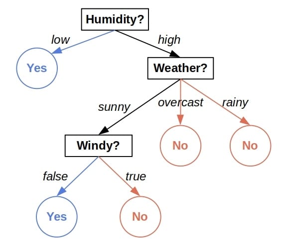
The internal nodes tell us which features to check, and the leaves reveal the tree’s prediction. How do they produce the predictions? Each leaf contains a subset of the training dataset. All its instances pass all the checks on the path from the root to the leaf. When predicting the outcome for a new object, we assign it the combined label of the training data that end in the same leaf as the instance. In the classification problems, it’s the associated subset’s majority class. Similarly, it’s the average value in regression.
2.1. Overfitting and Instability of Decision Trees
Decision trees suffer from two problems. First, they are prone to overfitting the data. Since accuracy improves with each internal node, training will tend to grow a tree to its maximum to improve the performance metrics. However, that deteriorates the tree’s generalization capability and usefulness on unseen data since it will start modeling the noise.
We can limit the tree’s depth beforehand, but there’s still the problem of instability. Namely, even small changes to the training data, such as excluding a few instances, can result in a completely different tree. That leaves us with the question of which tree to trust.
3. Random Forests
Random Forests address both issues. The idea is to construct multiple trees using different subsets of the training data and features for each tree in the forest. Then, we aggregate their predictions by outputting the majority vote or the average value.
The rationale is that an ensemble of models is likely more accurate than a single tree. So, even if a tree overfits its subset, we expect other trees in the forest to compensate for it. That’s why we use different subsets for each tree, to force them to approach the problem from different angles.
3.1. Example
Let’s say that we have the data:
![\[ \begin{matrix} \text{Weather} & \text{Humidity} & \text{Windy} & \text{PlayOutside} \\ \hline sunny & high & false & \textcolor{baeldungblue}{\text{Yes}} \\ sunny & low & false & \textcolor{baeldungblue}{\text{Yes}} \\ overcast & high & true & \textcolor{baeldungred}{\text{No}} \\ sunny & low & true & \textcolor{baeldungblue}{\text{Yes}} \\ overcast & low & false & \textcolor{baeldungblue}{\text{Yes}} \\ sunny & high & true & \textcolor{baeldungred}{\text{No}} \\ rainy & high & false & \textcolor{baeldungred}{\text{No}} \\ \hline \end{matrix}\]](/wp-content/ql-cache/quicklatex.com-73424a049fcbacff7501ebe23e270930_l3.svg "Rendered by QuickLaTeX.com")
We want to predict if a day is suitable for playing outside. Here’s an example of a forest with three trees:
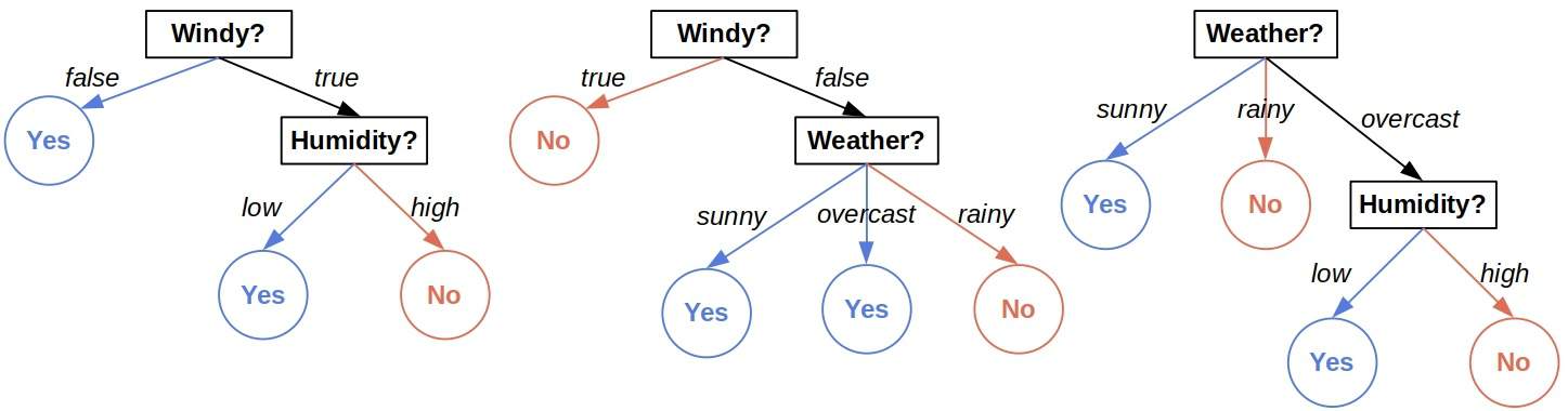
To classify the day:
![\[\langle Windy = true, Humidity = low, Weather = sunny \rangle\]](/wp-content/ql-cache/quicklatex.com-ddd3dab7abc5b32d2ecb65980feff97b_l3.svg "Rendered by QuickLaTeX.com")
we compute the predictions of all the trees and output the majority vote. The first and the third trees predict  , whereas the second predicts
  . So, the overall prediction is .
While combining the individual predictions, the most straightforward is to use the majority vote or the mean value. However, we can also weigh the predictions with the trees’ estimated accuracy scores so that the more precise trees get more influence.
3.2. Training Multiple Decision Trees
Although forests address the two issues of decision trees, there’s a question of complexity. Training a forest of  trees will take times longer than constructing a single tree. However, since we fit all the trees independently, we can build them simultaneously. That will speed up the training process but require infrastructure suitable for parallel computing.
Still, constructing a forest isn’t just a matter of spending more time. In addition to the hyper-parameters we need for a tree, we have to consider the number of trees in our forest,  . As a result, the number of hyper-parameter combinations to check during cross-validation grows.
3.3. The Interpretability Issue
Although a forest seems to be a more accurate model than a tree, the latter has a crucial advantage. A single tree is interpretable, whereas a forest is not. Humans can visualize and understand a tree, no matter if they’re machine learning experts or laypeople. That’s not the case with forests. They contain a lot of trees, so explaining how they output the aggregated predictions is very hard, if not impossible.
As the demand for interpretability grows stronger, less accurate but understandable models such as decision trees will still be present in real-world applications. Further, they are sometimes the only choice since the regulations forbid the models whose decisions the end-users can’t understand.
4. Conclusion
In this article, we talked about the difference between decision trees and random forests. A decision tree is prone to overfitting. Additionally, its structure can change significantly even if the training data undergo a negligible modification. Random forests contain multiple trees, so even if one overfits the data, that probably won’t be the case with the others. So, we expect an ensemble to be more accurate than a single tree and, therefore, more likely to yield the correct prediction. However, forests lose the interpretability a tree has.