

Learn through the super-clean Baeldung Pro experience:
>> Membership and Baeldung Pro.
No ads, dark-mode and 6 months free of IntelliJ Idea Ultimate to start with.
Learn through the super-clean Baeldung Pro experience:
>> Membership and Baeldung Pro.
No ads, dark-mode and 6 months free of IntelliJ Idea Ultimate to start with.
In this tutorial, we’ll give an overview of the Dijkstra and Bellman-Ford algorithms. We’ll discuss their similarities and differences.
Then, we’ll summarize when to use each algorithm.
Dijkstra’s algorithm is one of the SSSP (Single Source Shortest Path) algorithms. Therefore, it calculates the shortest path from a source node to all the nodes inside the graph.
Although it’s known that Dijkstra’s algorithm works with weighted graphs, it works with non-negative weights for the edges. We’ll explain the reason for this shortly.
In Dijkstra’s algorithm, we start from a source node and initialize its distance by zero. Next, we push the source node to a priority queue with a cost equal to zero.
After that, we perform multiple steps. In each step, we extract the node with the lowest cost, update its neighbors’ distances, and push them to the priority queue if needed. Of course, each of the neighboring nodes is inserted with its respective new cost, which is equal to the cost of the extracted node plus the edge we just passed through.
We continue to visit all nodes until there are no more nodes to extract from the priority queue. Then, we return the calculated distances.
The complexity of Dijkstra’s algorithm is  , where
  is the number of nodes, and
  is the number of edges in the graph.
In Dijkstra’s algorithm, we always extract the node with the lowest cost. We can prove the correctness of this approach in the case of non-negative edges.
Suppose the node with the minimum cost is  . Also, suppose we want to extract some other node
  that has a higher cost than . In other words, we have:

We can’t possibly reach with a lower cost if we extracted first. The reason behind this is that itself has a higher cost. Therefore, any path that takes us to starting from will have a cost equal to the cost of plus the distance from to . In other words, we are trying to prove that:

However, we already know that  is smaller than
  . Since
  has a non-negative weight, the last equation can never come true. Therefore, it’s always optimal to extract the node with the minimum cost.
So, we proved the optimality of Dijkstra’s algorithm. However, to do this, we assumed that all the edges have non-negative weights. Therefore, will always be non-negative as well.
When working with graphs that have negative weights, Dijkstra’s algorithm fails to calculate the shortest paths correctly. The reason is that might be negative, which will make it possible to reach from at a lower cost. Therefore, we can’t prove the optimality of choosing the node that has the lowest cost.
The main advantage of Dijkstra’s algorithm is its considerably low complexity, which is almost linear. However, when working with negative weights, Dijkstra’s algorithm can’t be used.
Also, when working with dense graphs, where is close to  , if we need to calculate the shortest path between any pair of nodes, using Dijkstra’s algorithm is not a good option.
The reason for this is that Dijkstra’s time complexity is . Since equals almost , the complexity becomes  .
.
When we need to calculate the shortest path between every pair of nodes, we’ll need to call Dijkstra’s algorithm, starting from each node inside the graph. Therefore, the total complexity will become  .
.
The reason why this is not a good enough complexity is that the same can be calculated using the Floyd-Warshall algorithm, which has a time complexity of  . Hence, it can give the same result with lower complexity.
As with Dijkstra’s algorithm, the Bellman-Ford algorithm is one of the SSSP algorithms. Therefore, it calculates the shortest path from a starting source node to all the nodes inside a weighted graph. However, the concept behind the Bellman-Ford algorithm is different from Dijkstra’s.
In the Bellman-Ford algorithm, we begin by initializing all the distances of all nodes with  , except for the source node, which is initialized with zero. Next, we perform
  steps.
In each step, we iterate over all the edges inside the graph. For each edge from node to , we update the respective distances of if needed. The new possible distance equals to the distance of plus the weight of the edge between and .
After steps, all the nodes will have the correct distance, and we stop the algorithm.
The Bellman-Ford algorithm’s time complexity is  , where is the number of vertices, and is the number of edges inside the graph. The reason for this complexity is that we perform steps. In each step, we visit all the edges inside the graph.
The Bellman-Ford algorithm assumes that after steps, all the nodes will surely have correct distances. Let’s prove this assumption.
Any acyclic path inside the graph can have at most nodes, which means it has edges. If a path has more than edges, it means that the path has a cycle because it has more than nodes. Therefore, it must visit the same node more than once.
We can guarantee that any shortest path won’t go through cycles. Otherwise, we could have removed the cycle, and gained a better path.
Going back to the Bellman-Ford algorithm, we can guarantee that after steps, the algorithm will cover all the possible shortest paths. Therefore, the algorithm is guaranteed to give an optimal solution.
So, we proved that the Bellman-Ford algorithm gives an optimal solution for the SSSP problem. However, the first limitation to our proof is that going through a cycle could improve the shortest path!
The only case this is correct is when we have a cycle that has a negative total sum of edges. In that case, we usually can’t calculate the shortest path because we can always get a shorter path by iterating one more time inside the cycle. Therefore, the term shortest path loses its meaning.
However, even if the graph has negative weights, our proof holds still as long as we don’t have negative cycles.
In fact, we can use the Bellman-Ford algorithm to check for the existence of negative cycles. The only update we need to do is to save the distances we calculated after performing steps. Next, we perform one more step (step number ) the same way we did before.
After that, we check whether we have a node that got a better path. If so, then we must have at least one negative cycle that is causing this node to get a shorter path.
The second limitation is related to undirected graphs. Although it’s true that we can always transform an undirected graph to a directed graph, Bellman-Ford fails to handle undirected graphs when it comes to negative weights.
As far as the Bellman-Ford algorithm is concerned, if the edge between and has a negative weight, we now have a negative cycle. The cycle is formed by going from to and back to , which has a weight equal to twice the edge between and .
The main advantage of the Bellman-Ford algorithm is its capability to handle negative weights. However, the Bellman-Ford algorithm has a considerably larger complexity than Dijkstra’s algorithm. Therefore, Dijkstra’s algorithm has more applications, because graphs with negative weights are usually considered a rare case.
As mentioned earlier, the Bellman-Ford algorithm can handle directed and undirected graphs with non-negative weights. However, it can only handle directed graphs with negative weights, as long as we don’t have negative cycles.
Also, we can use the Bellman-Ford algorithm to check the existence of negative cycles, as already mentioned.
Let’s take an example of a graph that has non-negative weights and see how Dijkstra’s algorithm calculates the shortest paths.
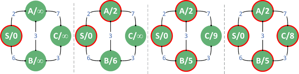
First, we push  to a priority queue and set its distance to zero. Next, we extract it, visit its neighbors, and update their distances. After that, we extract
  from the priority queue since it has the shortest distance, update its neighbors, and push them to the priority queue.
The next node to be extracted is  since it has the shortest path. As before, we update its neighbors and push them to the queue if needed. Finally, we extract
  from the queue, which now has its correct shortest path.
It’s worth noting that both and had their distances updated more than once. In the case of , we first set its distance equal to 6. However, when we extracted , we updated the distance of with the better path of distance 5.
The same holds for . When we extracted , we updated its distance to be equal to 9. However, when we extracted , we found a better path to , which has a distance equal to 8.
In each step, the only distance we were certain about is the lowest one. Therefore, we kept extracting it from the priority queue and updating its neighbors. When we didn’t have more nodes to extract from the priority queue, all the shortest paths had already been calculated correctly.
Now, let’s have a look at an example of a graph containing negative weights, but without negative cycles.
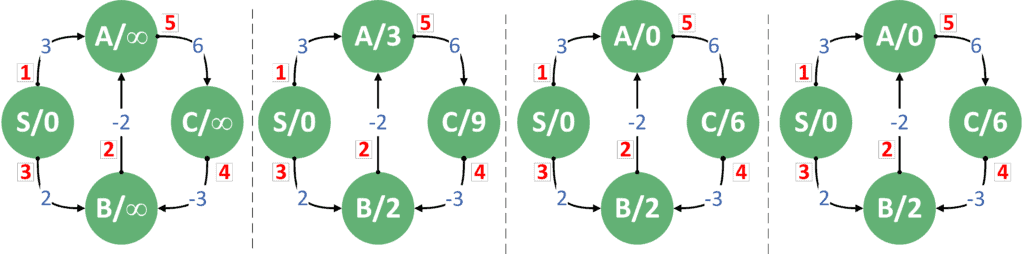
The red number near each edge shows its respective order. We performed three steps. In each step, we iterated over the edges by their order and updated the distances.
First, we updated the distance of from the first edge, updated the distance of from the third edge, and updated the distance of from the fifth edge. Next, we updated the distance of from the second edge and updated the distance of from the fifth edge. On the third step, we didn’t update any distances.
We can notice that performing any number of steps after the steps we already performed won’t change any distance. Therefore, we guarantee that the graph doesn’t contain negative cycles.
Now let’s look at an example that has negative cycles and explain how the Bellman-Ford algorithm detects negative cycles.
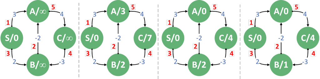
In the first step, we updated the distance of from the first edge, the distance of from the third edge, and the distance of from the fifth edge. Next, we updated the distance of from the second edge and the weight of from the fifth edge. Third, we updated the weight of from the fourth edge.
However, unlike the previous example, this example contains a negative cycle. The negative cycle is  because the sum of weights on this cycle is -1.
Let’s perform a few more iterations and see if the Bellman-Ford algorithm can detect it.
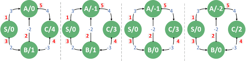
The first graph contains the resulting distances after performing the steps. If we performed one more step, we can notice that we update the distance of from the second edge and the distance of from the fourth edge. If we kept performing iterations, we’d notice that nodes , , and kept having lower distances because they are inside the negative cycle.
Therefore, since we have at least one node whose distance was updated, we can declare that the graph has negative cycles.
Take a look at the similarities and differences between Dijkstra’s and Bellman-Ford algorithms:
| Dijkstra | Bellman-Ford | |
|---|---|---|
| Non-Negative Weights |
Works correctly for directed and undirected graphs |
Works correctly for directed and undirected graphs |
| Negative Weights | Fails | Works correctly with directed graphs only |
| Negative Cycles | Fails | Can detect negative cycles in directed graphs |
| Time Complexity | |
|
As we can see, Dijkstra’s algorithm is better when it comes to reducing the time complexity. However, when we have negative weights, we have to go with the Bellman-Ford algorithm. Also, if we want to know whether the graph contains negative cycles or not, the Bellman-Ford algorithm can help us with that.
Just one thing to remember, in case of negative weights or even negative cycles, the Bellman-Ford algorithm can only help us with directed graphs.
In this tutorial, we provided an overview of Dijkstra’s and Bellman-Ford algorithms. We listed all the limitations, advantages, and disadvantages of each algorithm. Finally, we compared their strengths and weaknesses.