Bellman Ford Shortest Path Algorithm | Baeldung on Computer Science

1. Overview

The Bellman-Ford algorithm is a very popular algorithm used to find the shortest path from one node to all the other nodes in a weighted graph.

In this tutorial, we’ll discuss the Bellman-Ford algorithm in depth. We’ll cover the motivation, the steps of the algorithm, some running examples, and the algorithm’s time complexity.

2. Motivation

The Bellman-Ford algorithm is a single-source shortest path algorithm. This means that, given a weighted graph, this algorithm will output the shortest distance from a selected node to all other nodes.

It is very similar to the Dijkstra Algorithm. However, unlike the Dijkstra Algorithm, the Bellman-Ford algorithm can work on graphs with negative-weighted edges. This capability makes the Bellman-Ford algorithm a popular choice.

3. Why Are Negative Edges Important to Consider?

In graph theory, negative edges are more important as they can create a negative cycle in a given graph. Let’s start with a simple weighted graph with a negative cycle and try to find out the shortest distance from one node to another:

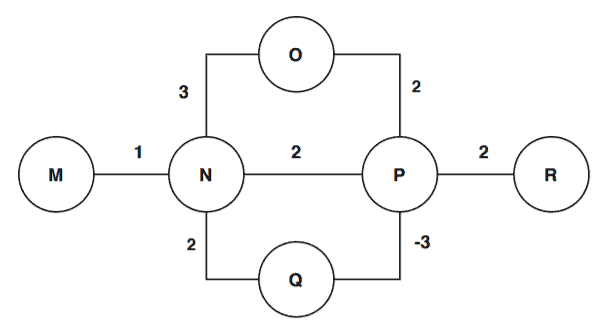
We’re considering each node as a city. We want to go to city R from city M.

There are three roads from the city M to reach the city R: MNPR, MNQPR, MNOPR. The road lengths are 5, 2, and 8.

But, when we take a deeper look, we see that there’s a negative cycle: NQP, which has a length of -1. So, each time we cover the path NQP, our road length will decrease.

This leads to us not being able to get an exact answer on the shortest path since repeating the road NQP infinite times would, by definition, be the least expensive route.

4. Steps of Bellman-Ford Algorithm

In this section, we’ll discuss the steps Bellman-Ford algorithm.

Let’s start with its pseudocode:

algorithm BellmanFord(G, S, W):
    // INPUT
    //    G = a directed graph with vertices V and edges E
    //    S = the starting vertex
    //    W = edge weights
    // OUTPUT
    //    Shortest path from S to all other vertices in G

    D <- a distance array with distances for each node
    D[S] <- 0
    R <- V - {S}
    C <- cardinality(V)

    // Initialize distances to infinity for all vertices except the starting vertex
    for vertex k in R:
        D[k] <- infinity 
    
    // Relax edges repeatedly
    for vertex i from 1 to (C - 1):
         for edge (e1, e2) in E:
             Relax the edge and update D with a new W if necessary
    // Check for negative weight cycles 
    for edge (e1, e2) in E: 
        if D[e2] > D[e1] + W[e1, e2]:
            print("Graph contains negative weight cycle")

This algorithm takes as input a directed weighted graph and a starting vertex. It produces all the shortest paths from the starting vertex to all other vertices.

Now let’s describe the notation that we used in the pseudocode. The first step is to initialize the vertices. The algorithm initially set the distance from starting vertex to all other vertices to infinity. The distance between starting vertex to itself is 0. The variable D[] denotes the distances in this algorithm.

After the initialization step, the algorithm started calculating the shortest distance from the starting vertex to all other vertices. This step runs $(|V| - 1 )$ times. Within this step, the algorithm tries to explore different paths to reach other vertices and calculates the distances. If the algorithm finds any distance of a vertex that is smaller then the previously stored value then it relaxes the edge and stores the new value.

Finally, when the algorithm iterates $(|V| - 1 )$ times and relaxes all the required edges, the algorithm gives a last check to find out if there is any negative cycle in the graph.

If there exists a negative cycle then the distances will keep decreasing. In such a case, the algorithm terminates and gives an output that the graph contains a negative cycle hence the algorithm can’t compute the shortest path. If there is no negative cycle found, the algorithm returns the shortest distances.

The Bellman-Ford algorithm is an example of Dynamic Programming. It starts with a starting vertex and calculates the distances of other vertices which can be reached by one edge. It then continues to find a path with two edges and so on. The Bellman-Ford algorithm follows the bottom-up approach.

5. An Example

5.1. A Graph Without Negative Cycle

Let’s try to visually understand how the Bellman-Ford algorithm works using a simple directed graph:

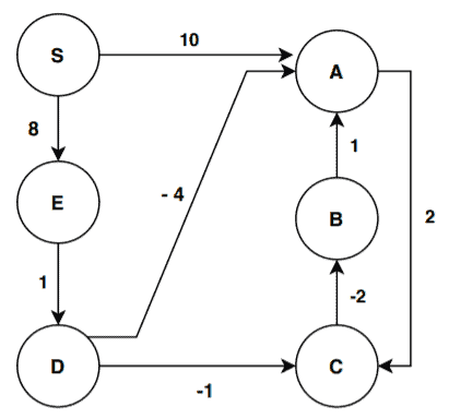
Assume that S is our starting vertex. We’re now ready to start with the initialization step of the algorithm:

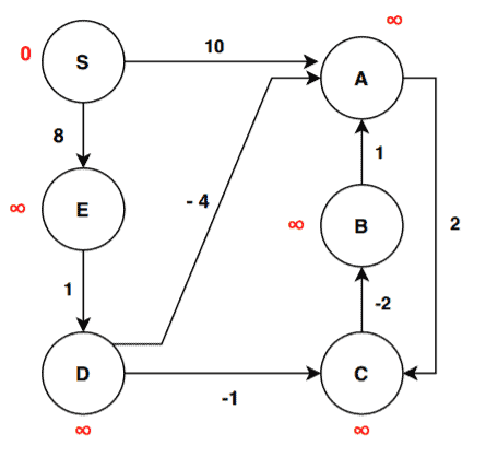
The values in red denote the distances. As we discussed, the distance from the starting node to the starting node is 0. The distance of all other vertices is infinite for the initialization step.

We’ve six vertices here. So, the algorithm will run five iterations for finding the shortest path and one iteration for finding a negative cycle if there exists any.

After initialization the graph, we can now proceed to the first iteration:

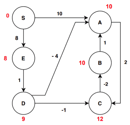
We can see some of the vertices have different distance values than the initialization step. Let’s find out how the distance values are being updated. The algorithm selects each edge and passes it to the function Relax(). First, for the edge (S, A) let’s see how Relax(S, A) function works. It first checks the condition:

$D[A] > D[S] + W[S, A] \implies \infty > 0 + 10 \implies \infty > 10 \implies True$

The edge (S, A) satisfies the checking condition, therefore, the vertex A gets a new distance:

$D[A] = D[S] + W[S, A] \implies D[A] = 0 + 10 = 10$

Now the new distance value of vertex A is 10. Our second edge is (A, B). Again this edge will go through the same step. The algorithm passes this edge to Relax() and the edge go through the checking step:

$D[B] > D[A] + W[A, B] \implies \infty > 10 + 2 \implies \infty > 12 \implies True$

The edge (A, B) passes the check condition and gets the new value:

$D[B] = D[A] + W[A, B] \implies D[B] = 10 + 2 = 12$

In this way, the algorithm passes all the edges to Relax() and if the edge satisfies then the vertex gets the new value. One important point here is the sequence of edges that are considered. Depending on the sequence of edges, one might get different distance values for vertices after an iteration. This is absolutely fine. To avoid any confusion, we’re listing out the order of edges that we followed for this example:

(S, A) -> (S, E) -> (A, C) -> (B, A) -> (C, B) -> (D, C) -> (D, A) -> (E, D)

Now we’re done with the first iteration. Let’s see how the graph changes after the second iteration:

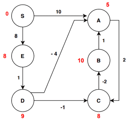
We can see from iteration 1, there are two changes in distance value. Let’s investigate further and go through our edge list one by one. The edges (S, A), (S, E), (A, C), (B, A), (C, B), (E, D) don’t satisfy the check condition. Therefore there won’t be any changes to the distance values. The edges (D, C), and (D, A) satisfy the condition. For edge (D, C):

$D[C] > D[D] + W[D, C] \implies 12 > 9 + (-1) \implies 12 > 8 \implies True$

Therefore the algorithm updates the new value of the vertex C:

$D[C] = D[D] + W[D, C] \implies D[C] = 9 + (-1) = 8$

Let’s check the edge (D, A):

$D[A] > D[D] + W[D, A] \implies 10 > 9 + (-4) \implies 10 > 5 \implies True$

The algorithm updates the new value of the vertex A:

$D[A] = D[D] + W[D, A] = 9 + (-4) = 5$

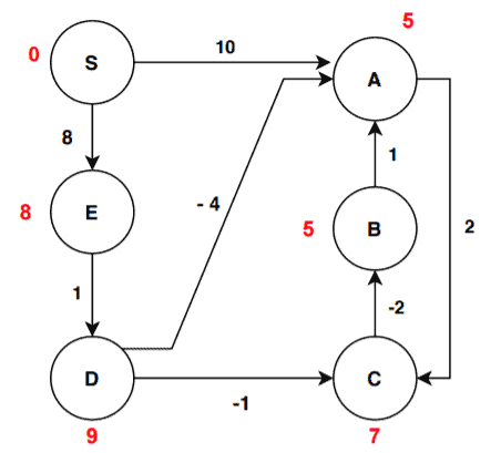
We’re now ready to move to the third iteration:

In the third iteration, there are two changes in distance values from the last iteration. The edges (S, A), (S, E), (B, A), (D, C), (D, A), (E, D) don’t satisfy the check condition hence remains unchanged. The edges (A, C) and (C, B) satisfies the condition. For edge (A, C):

$D[C] > D[A] + W[A, C] \implies 8 > 5 + 2 \implies 8 > 7 \implies True$

Therefore, the new value of the vertex C is updated:

$D[C] = D[A] + W[A, C] = 5 + 2 = 7$

Again for the edge (C, B):

$D[B] > D[C] + W[C, B] \implies 10 > 7 + (-2) \implies 10 > 5 \implies True$

Hence the new value of B is stored:

$D[B] = D[C] + W[C, B] = 7 + (-2) = 5$

Let’s proceed to the fourth iteration now:

There are no updates in the distance values of vertices after the fourth iteration. This means the algorithms produce the final result. Now, we mentioned that we need to run this algorithm for 5 interactions. But in this case, we got our result after 4.

In general $(|V| - 1)$ is the highest number of iterations that we need to run in case the distance values of the consecutive iterations are not stable. In this case, we got the same values for two consecutive iterations hence the algorithm terminates.

5.2. A Graph With Negative Cycle

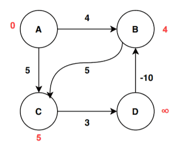
In this section, we’ll take another weighted directed graph that has a negative cycle. We’ll run the Bellman-Ford algorithm to see whether the algorithm detects the negative cycle or not:

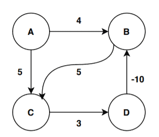
The graph has 4 vertices. We’re considering the vertex A as the starting vertex here. The algorithm expects to iterate 3 times for calculation of shortest distance and one more time to check for the negative cycle. The edge order we’re going to follow here is: (D, B) -> (C, D) -> (A, C) -> (A, B) -> (B, C)

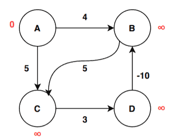
The first step is to initialize the graph:

As we’re done with the initialization, we can proceed to the first iteration:

After the first iteration, we can see changes in the distance value of B and C. From the vertex A, the edge weights are directly assigned to vertex B and C to update their distance value. For edge (A, C):

$D[C] > D[A] + W[A, C] \implies \infty > 0 + 5 \implies \infty > 5 \implies True$

Therefore, the new value of the vertex C is updated:

$D[C] = D[A] + W[A, C] = 0 + 5 = 5$

Similarly for edge (A, B):

$D[B] > D[A] + W[A, B] \implies \infty > 0 + 4 \implies \infty > 4 \implies True$

The algorithm stores the new value of B:

$D[B] = D[A] + W[A, B] = 0 + 4 = 4$

Let’s see how the value changes after the second iteration:

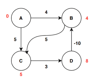
After the second iteration, the distance value of the vertex D is updated by the algorithm by relaxing the edge (C, D):

$D[D] > D[C] + W[C, D] \implies \infty > 5 + 3 \implies \infty > 8 \implies True$

Therefore, the new value of the vertex C is updated:

$D[D] = D[C] + W[C, D] = 5 + 3 = 8$

After third iteration, the values are again getting changed:

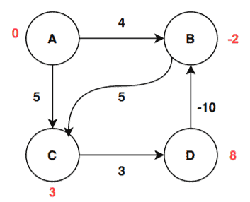
Here there are two updates. One for the vertex B and another for vertex C. The update for vertex B is done by relaxing the edge (D, B):

$D[B] > D[D] + W[D, B] \implies 4 > 8 + (-10) \implies 4 > -2 \implies True$

Therefore, the new value of the vertex B is updated:

$D[B] = D[D] + W[D, B] = 8 + (-10) = -2$

The algorithm updated the value for vertex B by relaxing the edge (B, C):

$D[C] > D[B] + W[B, C] \implies 5 > (-2) + 5 \implies 5 > 3 \implies True$

The value of C is updated and stored:

$D[C] = D[B] + W[B, C] = (-2) + 5 = 3$

We’re done with the maximum required iterations. Now let’s iterate one last time to decide whether the graph has a negative cycle or not:

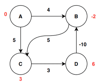
We can see there is a change in value for vertex D. The change happens as the algorithm relax the edge (C, D):

$D[D] > D[C] + W[C, D] \implies 8 > 3 + 3 \implies 8 > 6 \implies True$

The value of C is updated and stored:

$D[C] = D[C] + W[C, D] = 3 + 3 = 6$

The distance values are not stable even after the maximum number of iterations. Therefore, in this case, the algorithms return that the graph contains a negative weighted cycle, and hence it is not possible to calculate the shortest path from the starting vertex to all other vertices in the given graph.

6. Time Complexity Analysis

To end, we’ll look at Bellman-Ford’s time complexity.

First, the initialization step takes $O(V)$ .

Then, the algorithm iterates $(|V| - 1)$ times with each iteration taking $O(1)$ time.

After $(|V| - 1)$ interactions, the algorithm chooses all the edges and then passes the edges to Relax(). Choosing all the edges takes $O(E)$ time and the function Relax() takes $O(1)$ time.

Therefore the complexity to do all the operations takes $O(VE)$ time.

Within the Relax() function, the algorithm takes a pair of edges, does a checking step, and assigns the new weight if satisfied. All these operations take $O(E)$ times.

Thus the total time of the Bellman-Ford algorithm is the sum of initialization time, for loop time, and Relax function time. In total, the time complexity of the Bellman-Ford algorithm is $\textbf{O(VE)}$ .

7. Conclusion

In this article, we’ve discussed the Bellman-Ford algorithm in detail. We’ve discussed the steps of the algorithm and run the algorithm on two different graphs to give the reader a complete understanding. Also, we examined why negative edges are important to consider.

Finally, we analyzed the time complexity of the algorithm.

Full Archive

About Baeldung

Core Concepts

Operating Systems

Artificial Intelligence

Graph Theory

Latex

1. Overview

2. Motivation

3. Why Are Negative Edges Important to Consider?

4. Steps of Bellman-Ford Algorithm

5. An Example

5.1. A Graph Without Negative Cycle

5.2. A Graph With Negative Cycle

6. Time Complexity Analysis

7. Conclusion