Bias Update in Neural Network Backpropagation | Baeldung on Computer Science

1. Introduction

In this tutorial, we’ll explain how weights and bias are updated during the backpropagation process in neural networks. First, we’ll briefly introduce neural networks as well as the process of forward propagation and backpropagation. After that, we’ll mathematically describe in detail the weights and bias update procedure.

The purpose of this tutorial is to make clear how bias is updated in a neural network in comparison to weights.

2. Neural Networks

Neural networks are algorithms explicitly designed to simulate biological neural networks. In general, the idea was to create an artificial system that behaves like the human brain. Depending on the type of network, neural networks are based on interconnected neurons. There are many types of neural networks, but we can broadly divide them into three classes:

The main distinction between them is the type of neurons that comprise them, as well as the manner in which information flows through the network. In this article, we’ll explain backpropagation using regular neural networks.

3. Artificial Neurons

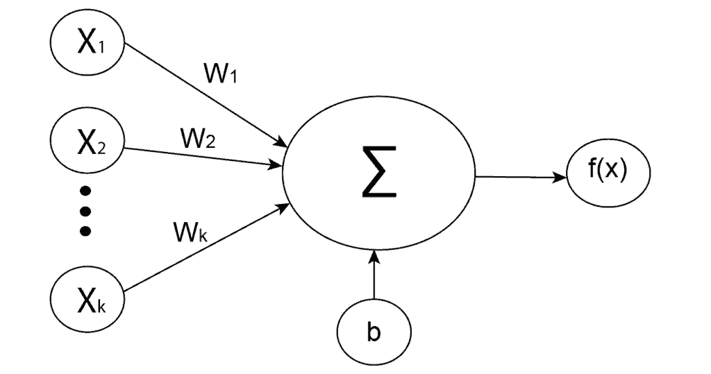
Artificial neurons serve as the foundation for all neural networks. They are units modeled after biological neurons. Each artificial neuron receives inputs and produces a single output, which we also send to a network of other neurons. Inputs are usually numeric values from a sample of external data, but they can also be other neurons’ outputs. The neural network’s final output neurons represent the value that defines prediction.

To obtain the output of the neuron, we need to compute the weighted sum of all the inputs and weights of the connections. Then we add bias to the sum and use the activation function. Mathematically, we define the weighted sum as:

(1) $\begin{align*} z = w_{1}x_{1} + w_{2}x_{2} + ... + w_{k}x_{k} + b, \end{align*}$

where $w_{i}$ are weights, $x_{i}$ are inputs and $b$ bias. After that, an activation function $f$ is applied to the weighted sum $z$ , which represents the final output of the neuron:

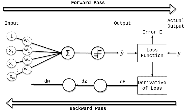
4. Forward Propagation and Backpropagation

During the neural network training, there are two main phases:

Forward propagation
Backpropagation

4.1. Forward Propagation

First comes forward propagation which means that the input data is fed in the forward direction through the network. Overall, this process
covers the data flow from the initial input, passing by every layer in the network, and finally the computation of the prediction error. This is a typical procedure in feed-forward neural networks but for some other networks, such as RNNs, the forward propagation is slightly different.

To conclude, forward propagation is a process that starts with input data and ends when the error of the network is calculated.

4.2. Backpropagation

After forward propagation comes backpropagation and it’s certainly the essential part of the training. In brief, it’s a process of fine-tuning the weights of a network based on the errors or loss obtained in the previous epoch (iteration). Proper weight tuning ensures lower error rates while increasing the model’s reliability by enhancing its generalization.

Initially, we have a neural network that doesn’t give accurate predictions because we haven’t tuned the weights yet. The point of backpropagation is to improve the accuracy of the network and at the same time decrease the error through epochs using optimization techniques.

There are many different optimization techniques that are usually based on gradient descent methods but some of the most popular are:

In brief, gradient descent is an optimization algorithm that we use to minimize loss function in the neural network by iteratively moving in the direction of the steepest descent of the function. Therefore, in order to find the direction of the steepest descent, we need to calculate gradients of the loss function with respect to weights and bias. After that, we’ll be able to update weights and bias using negative gradients multiplied by the learning rate:

4.3. Weights Update

To begin with, let’s consider the snippet of the neural network presented below, where $l$ indicates $l$ -th layer, $a$ is the activation column-vector or vector with neurons and $W$ is the weight matrix:

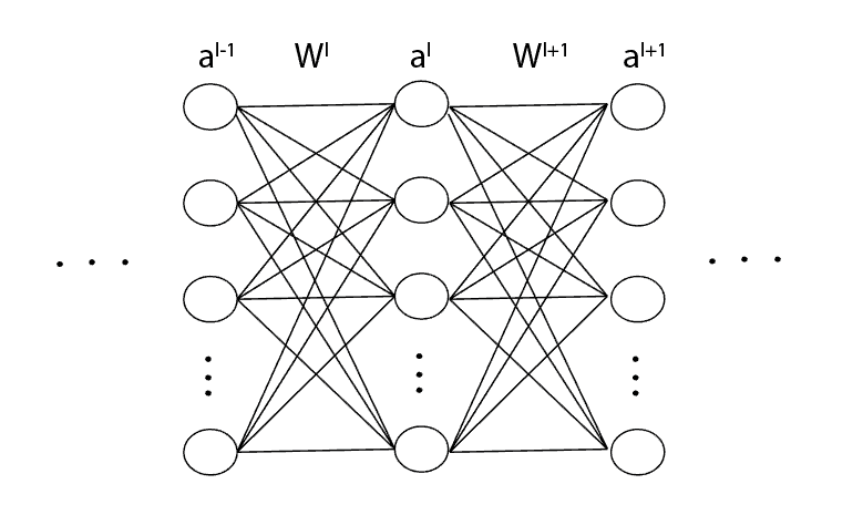
Following neural network definition, the formula for one specific neuron $a_{k}^{l}$ , in the $l$ -th layer is

(2) $\begin{align*} a_{k}^{l} &= \sigma(z_{k}^{l})\\ z_{k}^{l} &= w_{k1}^{l}a_{1}^{l-1} + w_{k2}^{l}a_{2}^{l-1} + ... + w_{kn}^{l}a_{n}^{l-1} + b_{k}^{l}, \end{align*}$

where $\sigma$ is activation function, $w$ weights and $b$ bias.

Firstly, if we want to update one specific weight $w_{kj}^{l}$ , we would need to calculate the derivative of the cost function $C$ with respect to that particular weight, or

(3) $\begin{align*} \frac{\partial C}{\partial w_{kj}^{l}}. \end{align*}$

Now, if we apply the chain rule and extend the derivative, we’ll get

(4) $\begin{align*} \frac{\partial C}{\partial w_{kj}^{l}} = \frac{\partial C}{\partial z_{k}^{l}}\frac{\partial z_{k}^{l}}{\partial w_{kj}^{l}} = \frac{\partial C}{\partial a_{k}^{l}}\frac{\partial a_{k}^{l}}{\partial z_{k}^{l}}\frac{\partial z_{k}^{l}}{\partial w_{kj}^{l}} \end{align*}$

or consequently presented graphically:

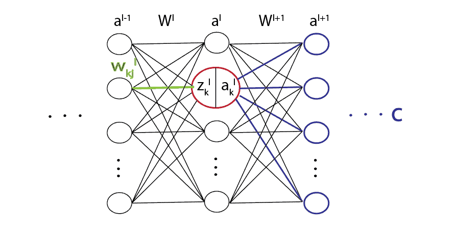
Basically, using the chain rule, we break a large problem into smaller ones and solve them one by one. Using the chain rule again, we would also need to break $\frac{\partial C}{\partial a_{k}^{l}}$ even further into:

(5) $\begin{align*} \frac{\partial C}{\partial w_{kj}^{l}} =& \frac{\partial C}{\partial z_{k}^{l}}\frac{\partial z_{k}^{l}}{\partial w_{kj}^{l}} = \frac{\partial C}{\partial a_{k}^{l}}\frac{\partial a_{k}^{l}}{\partial z_{k}^{l}}\frac{\partial z_{k}^{l}}{\partial w_{kj}^{l}} = \\ =& (\sum_{m}\frac{\partial C}{\partial z_{m}^{l+1}}\frac{\partial z_{m}^{l+1}}{\partial a_{k}^{l}})\frac{\partial a_{k}^{l}}{\partial z_{k}^{l}}\frac{\partial z_{k}^{l}}{\partial w_{kj}^{l}} = \\ \stackrel{(2)}{=}& (\sum_{m}\frac{\partial C}{\partial z_{m}^{l+1}}w_{mk}^{l+1})\sigma^{'}(z_{k}^{l})a_{j}^{l-1} \end{align*}$

4.4. Error Signal

After that, let’s define the error signal of a neuron $k$ in layer $l$ as

(6) $\begin{align*} \delta_{k}^{l} = \frac{\partial C}{\partial z_{k}^{l}}. \end{align*}$

From the equation (5), we also can extract the recurrent expression

(7) $\begin{align*} \frac{\partial C}{\partial z_{k}^{l}} = (\sum_{m}\frac{\partial C}{\partial z_{m}^{l+1}}w_{mk}^{l+1})\sigma^{'}(z_{k}^{l}), \end{align*}$

or using the error signal notation

(8) $\begin{align*} \delta_{k}^{l} = (\sum_{m}\delta_{m}^{l+1}w_{mk}^{l+1})\sigma^{'}(z_{k}^{l}), \end{align*}$

This recurrent relation propagates to the last layer in the network and the error signal of a neuron $k$ in the last layer $L$ is equal to

(9) $\begin{align*} \delta_{k}^{L} =\frac{\partial C}{\partial z_{k}^{L}} = \frac{\partial C}{\partial a_{k}^{L}}\frac{\partial a_{k}^{L}}{\partial z_{k}^{L}} = \frac{\partial C}{\partial a_{k}^{L}}\sigma^{'}(z_{k}^{L}). \end{align*}$

Finally, everything is explained and we can substitute the error signal (6) in the initial derivative (5)

(10) $\begin{align*} \frac{\partial C}{\partial w_{kj}^{l}} = \delta_{k}^{l}a_{j}^{l-1}. \end{align*}$

Lastly, we update the weight $w_{kj}^{l}$ as

(11) $\begin{align*} w_{kj}^{l} = w_{kj}^{l} - \alpha \delta_{k}^{l}a_{j}^{l-1}. \end{align*}$

where $\alpha$ is the learning rate.

4.5. Bias Update

Generally, a bias update is very similar to a weight update. Due to the derivative rule that for every $x$

(12) $\begin{align*} x^{'} = \frac{\partial x}{\partial x} = 1, \end{align*}$

we also have that for any $a \neq x$

(13) $\begin{align*} \frac{\partial (x + a)}{\partial x} = 1 + 0 = 1. \end{align*}$

Likewise, for $k$ -th bias in layer $l$ , we have that

(14) $\begin{align*} \frac{\partial C}{\partial b_{k}^{l}} = \frac{\partial C}{\partial z_{k}^{l}}\frac{\partial z_{k}^{l}}{\partial b_{k}^{l}} \stackrel{(2)}{=} \frac{\partial C}{\partial z_{k}^{l}} \cdot 1 \stackrel{(6)}{=} \delta_{k}^{l}. \end{align*}$

Now, similarly to weight update (11), we can update bias as

(15) $\begin{align*} b_{k}^{l} = b_{k}^{l} - \alpha \delta_{k}^{l}. \end{align*}$

5. Conclusion

In this article, we briefly explained the neural network’s terms with artificial neurons, forward propagation, and backward propagation. After that, we provided a detailed mathematical explanation of how bias is updated in neural networks and what is the main difference between bias update and weight update.

This article has both theoretical and mathematical parts and therefore requires some prior knowledge about derivatives.

Full Archive

About Baeldung

Core Concepts

Operating Systems

Artificial Intelligence

Graph Theory

Latex