Choosing a Learning Rate | Baeldung on Computer Science

1. Introduction

When we start to work on a Machine Learning (ML) problem, one of the main aspects that certainly draws our attention is the number of parameters that a neural network can have.

Some of these parameters are meant to be defined during the training phase, such as the weights connecting the layers. But others, such as the learning rate or weight decay, should be defined by us, the developers.

We’ll use the term hyperparameters to refer to the parameters that we need to define. The process of adjusting them will be called fine-tuning.

Currently, some ML datasets have millions of training instances or even billions. If we choose a wrong value for any of these parameters, this could make our model converge in more time than needed, reaching a non-optimal solution, or even worse, to a scenario where the convergence never occurs.

In this tutorial, we’ll focus only on the learning rate, illustrating different approaches to define its value to achieve a satisfactory model.

2. Theoretical Background

Before we dive into the mathematical foundations of neural networks to precisely understand the role of the learning rate, we should briefly review some Generalization Theory concepts.

In this way, we’ll be able to evaluate different methods for the definition of this parameter and the reason behind this concern to optimize its value.

2.1. Generalization Theory

What is a good model in Machine Learning? How can we have a system that performs well both on the training set and on never-seen data?

To answer these questions, we should understand the model’s ability to generalize, which is closely related to the learning rate definition, among other hyperparameters.

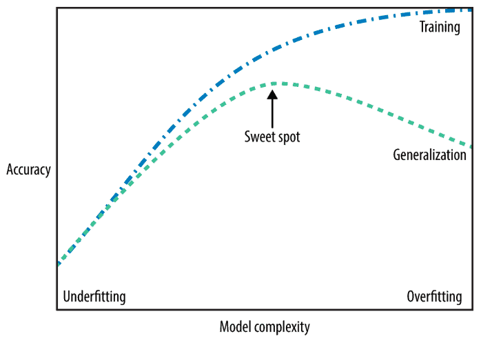
When our model is too simple and cannot correctly classify both training and testing samples, we say that underfitting happened.

But when our model can correctly accurately classify the samples of the training set but performs poorly on new data, we say that our model is overfitting. This is because the system became so complex and learned features that are strictly related to the training set without the capacity of generalization.

We desire to achieve the sweet spot, where the accuracy might not be at its higher level for the training set but performs properly on new data that was not used for training:

2.2. Back to Basics: Gradient Descent

We’ll briefly discuss how Gradient-Based optimization works until we reach the point where the learning rate comes into place. After that, we’ll describe different methods to define its value.

In Deep Learning, most algorithms imply an optimization problem. We usually want to minimize some function $f(\textbf{x})$ that we call loss function or error function.

To reach this minimum point, we calculate the derivative of the function $y = f(x)$ , where $x$ and $y$ are real numbers:

(1) $\begin{equation*} f'(x) = \frac{dy}{dx} \end{equation*}$

We won’t explain how to calculate the derivative, but you can check a simple example.

The derivative $f'(x)$ represents the slope of $f(x)$ at the point $x$ . To rephrase it: how much we should change the input to obtain the corresponding change in the output:

(2) $\begin{equation*} f(x+\epsilon) \approx f(x) + \epsilon f'(x). \end{equation*}$

We define Gradient Descent as the process of calculating the derivative at different points, taking small steps in the opposite direction of the current derivative.

Following this strategy, we can reach the local or global minimum of a function.

2.3. The Multiple Inputs Case

In the previous section, we only had a function $y = f(x)$ to calculate the derivatives.

But in Deep Learning, the problems can easily have multiple inputs with more complex models. So how can we calculate the derivative in this case?

We should calculate the partial derivatives for each input variable. Let’s suppose we have as input $x_{1},x_{2},..x_{i}$ , we’ll represent the partial derivative of $f$ if we change the variable $x_{i}$ at the point $x$ as:

(3) $\begin{equation*} \frac{\partial}{\partial x_{i}} f(x) \end{equation*}$

We can group all the partial derivatives in a vector $\triangledown_{x}f(x)$ that we call gradient.

To minimize $f$ we’ll move in the direction of the negative gradient to a new point $x'$ defined as:

(4) $\begin{equation*} x'=x - \epsilon \triangledown_{x}f(x) \end{equation*}$

Finally, we reached the learning rate, which is represented by $\epsilon$ .

The learning rate will define the size of the step taken in each iteration during the gradient descent calculation, as we try to find the minimum of a loss function.

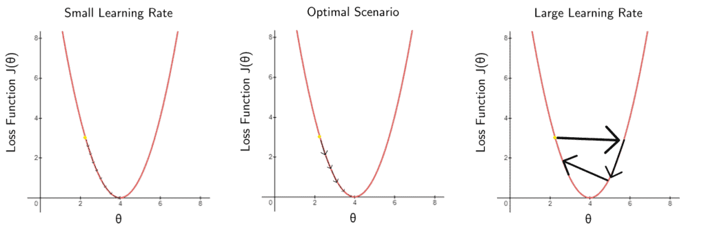
2.4. Impact of a Bad Learning Rate

What can go wrong if we choose the wrong learning rate?

One of the two things: i) we’ll have very slow progress since we’re taking minimal steps to update the weights, or ii) we’ll never even reach the desired point since we might define a large rate that will make the model bounce across the loss function without any convergence:

3. How to Choose the Learning Rate

To avoid the aforementioned problems, we can implement different methods to define the learning rate during the training phase.

In the following examples, we’ll consider a cost function $J(\theta)$ parametrized by $\theta \in \mathbb{R}$ . The learning rate will be represented by $\alpha$ , the gradient by $g$ , and the weights by $w$ .

3.1. Learning Rate Annealing

One of the most simple approaches that we can implement is to have a schedule to reduce the learning rate as the epochs of our training progress.

This strategy takes advantage of the fact that we want to explore the space with a higher learning rate initially, but as we approach the final epochs, we want to refine our result to get closer to the minimum point.

For example, if we want to train our model for 1000 epochs, we might start with a learning rate of 0.1 until epoch 400. After that, we can reduce the learning rate to 0.01 until epoch 700. Lastly, we can train the last epochs with a 0.001 learning rate.

We can use a larger number of steps and variations for this hyperparameter if we have a high-dimensional problem.

3.2. Root Mean Square Propagation (RMSProp)

RMSProp is an optimizer that will update the learning rate during the iterations, based on the fact that early updates should have less weight in later updates.

Simply put, the learning rate will be divided by the average of square gradients in an exponentially decaying approach, preventing abrupt changes:

(5) $\begin{equation*} m_{t} = \beta m_{t-1} + (1-\beta) g_{t}^{2} \end{equation*}$

In which, $m_{t}$ represents the moving average of squared gradients.

With RMSProp, we have a moving average parameter, represented by $\beta$ that is set to 0.9 by default.

After calculating the moving average, we can update the weights, in which $\epsilon$ is a constant to prevent division by zero:

(6) $\begin{equation*} w_{t} = w_{t-1} - \frac{\alpha}{\sqrt{m_{t}+ \epsilon}} g_{t}} \end{equation*}$

3.3. Adam

We can consider the Adaptive Moment Estimation (Adam) method as a combination of RMSProp and the traditional gradient descent. It also uses the moving average of squared gradients combined with the moving average of the gradient:

The first is the estimate of the first moment $m_{t}$ :

(7) $\begin{equation*} m_{t} = \beta_{1} m_{t-1} + (1 - \beta_{1}) g_{t} \end{equation*}$

The second is the estimate of the second moment, the uncentered variance:

(8) $\begin{equation*} v_{t} = \beta_{2} v_{t-1} + (1 - \beta_{2}) g_{t}^{2} \end{equation*}$

The default values for $\beta_{1}$ and $\beta_{2}$ are 0.9 and 0.999, respectively. We should initialize both $m_{t}$ and $v_{t}$ as 0’s, and for this reason the moments are biased towards zero.

To correct this error, we use the following values:

(9) $\begin{equation*} \hat{m}_{t}=\frac{m_{t}}{1 - \beta_{1}^t} \end{equation*}$

(10) $\begin{equation*} \hat{v}_{t}=\frac{v_{t}}{1 - \beta_{2}^t} \end{equation*}$

And we can finally elaborate on the final rule to update the weights using Adam optimizer:

(11) $\begin{equation*} w_{t+1} = w_{t} - \frac{\alpha}{\sqrt{\hat{v}_{t}}+\epsilon} \hat{m}_{t} \end{equation*}$

3.4. Adagrad

The main idea of the Adagrad strategy is that it uses a different learning rate for each parameter.

The immediate advantage is to apply a small learning rate for parameters that are frequently updated and a large learning rate for the opposite scenario.

In this way, if our data is spread across the space in a sparse way, Adadelta can be used. The update rule for this method includes a matrix $G_{t}$ containing the sum of squared gradients only considering the $i-th$ parameter:

(12) $\begin{equation*} w_{t+1,i} = w_{t,i} - \frac{\alpha}{\sqrt{G_{t,ii}+\epsilon}} g_{t,i} \end{equation*}$

3.5. Adadelta

We can also use Adadelta to adjust the learning rate. The difference between this method and Adagrad is that here we won’t accumulate all past gradients.

We’ll have a parameter $\gama$ , usually set to 0.9, that affects our calculation of the moving average:

(13) $\begin{equation*} E[g^{2}]_{t} = \gamma E[g^{2}]_{t-1} + (1-\gamma) g_{t}^{2} \end{equation*}$

(14) $\begin{equation*} w_{t+1} = w_{t} - \frac{\alpha}{\sqrt{E[g^{2}]_{t}+\epsilon}} g_{t} \end{equation*}$

One of the main advantages of Adadelta is that we don’t need to set a default learning rate, reducing the number of hyperparameters to be manually tuned.

3.6. Population-Based Training (PBT)

We can also use a method developed by Deep Mind, which consists of a different approach of a random search associated with hand-tuning.

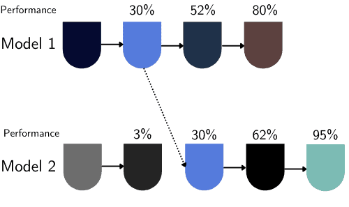
The principle of PBT is that we don’t need to continue training a model which is performing poorly compared to others.

Suppose we suppose that we have only two models with different hyperparameters being trained, which includes the learning rate. If Model 1 presents an accuracy of 30% and Model 2 has a 3% accuracy, there is no reason to continue to train Model 2 with those hyperparameters.

So we replace Model 2 with the current stage of Model 1 and continue to explore different values:

4. Examples of Different Learning Rates

To exemplify the effect of using the same optimizer with different learning rates, we used the Adam algorithm to train a neural network that recognizes dog breeds among 120 classes.

We can easily see the influence of using three different learning rates with the same strategy:

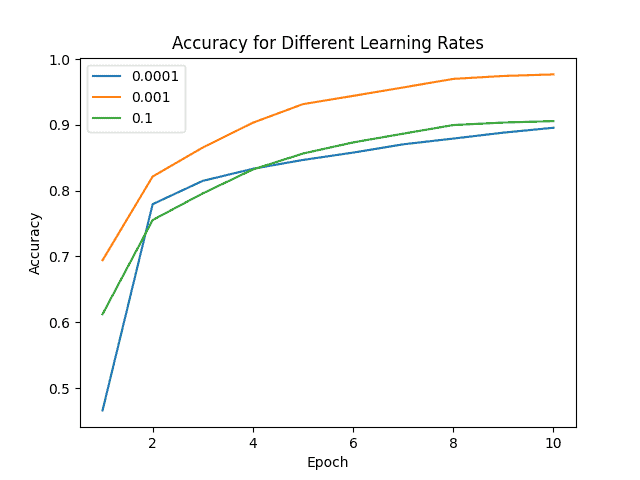
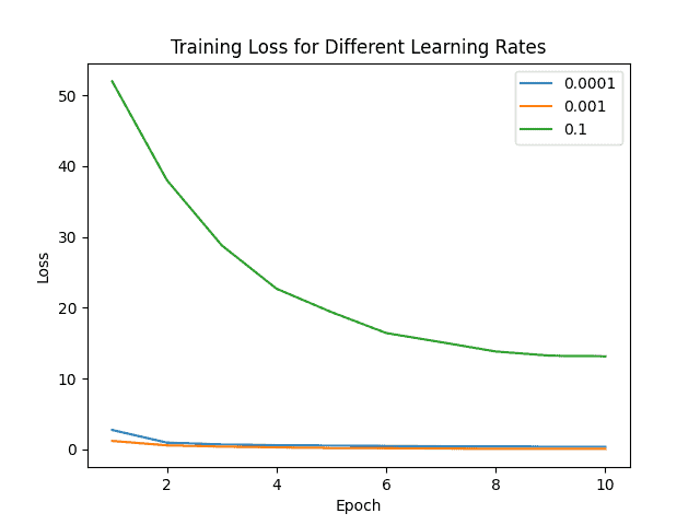
We can clearly see how the learning rate of 0.001 outperforms the other scenarios, proving that for this case, it is the optimal value.

Finally, we also compared the performance of training using the same neural network architecture with different approaches to defining the learning rate:

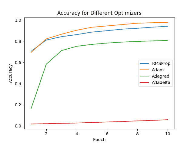
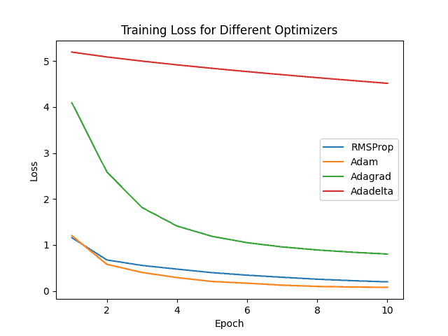
It is relevant to highlight that we used the same value for learning rate in all scenarios with the parameters configured to its default values.

To recognize dog breeds, the Adam optimizer had the higher accuracy and lower loss, illustrating that it should be considered the first strategy or guess to obtain a satisfactory model.

5. Conclusion

In this article, we discussed different strategies to update the weights during the training phase of a Machine Learning model. The example demonstrated how a different learning rate or strategy could dramatically affect our output for the training and test stages.

Although we cannot develop a strict rule to solve all problems and choose the optimal values for the learning rate, we can take advantage of well-established approaches. In this way, we’d be able to have a decent first guess, and from that point, we’d be able to fine-tune the model.

Full Archive

About Baeldung

Core Concepts

Operating Systems

Artificial Intelligence

Graph Theory

Latex