

Learn through the super-clean Baeldung Pro experience:
>> Membership and Baeldung Pro.
No ads, dark-mode and 6 months free of IntelliJ Idea Ultimate to start with.
Last updated: March 18, 2024
Learn through the super-clean Baeldung Pro experience:
>> Membership and Baeldung Pro.
No ads, dark-mode and 6 months free of IntelliJ Idea Ultimate to start with.
In this tutorial, we’ll cover significant differences between regular neural networks, also known as fully connected neural networks, and convolutional neural networks. We use these two types of networks to solve complex problems in various fields such as image recognition, object detection, building forecasting modes, and others.
Although we might use them both to solve the same problem, there are some pros and cons to choosing the specific one. Therefore, besides architectural differences, we’ll also cover the differences in their applications.
Neural networks are algorithms created explicitly to simulate biological neural networks. Generally, the idea was to create an artificial system that would function like the human brain. Neural networks are based on interconnected neurons depending on the type of network. There are many types of neural networks, but broadly, we can divide them into three classes:
The main difference between them lies in the types of neurons that make them up and how information flows through the network.
Regular or fully connected neural networks (FCNN) are the oldest and most common type of neural networks. Basically, the first mathematical model of a multilayer neural network, called multilayer perceptron (MLP), was a fully connected neural network.
To understand this type of network, we would need to explain some of its components.
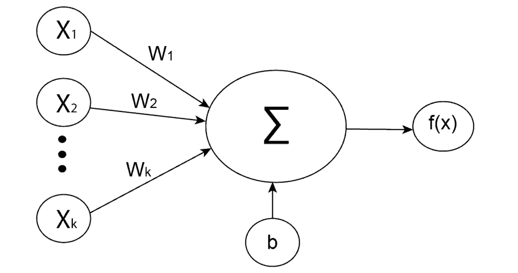
Artificial neurons are the base of all neural networks. They are units inspired by biological neurons. Each artificial neuron receives inputs and generates a single output that we transmit to multiple other neurons. Inputs are typically numeric values from a sample of external data, but they can also be the outputs of other neurons. The outputs of the final output neurons of the neural network represent the value that defines prediction.
In order to get the output of the neuron, we need to calculate the weighted sum of all the inputs and weights of the connections. After that, we add bias to the sum and apply the activation function. Mathematically, we define the weighted sum as:
(1) 
where  are weights,
  are inputs and
  bias. After that, an activation function is applied to the weighted sum
  , which represents the final output of the neuron:
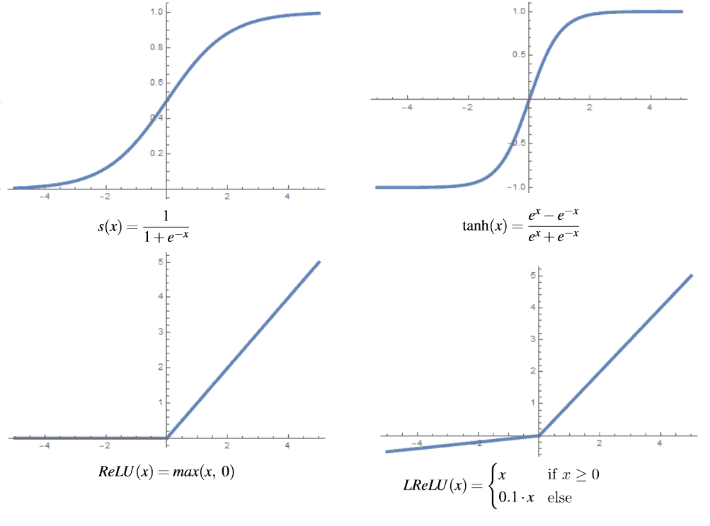
There are several types of activation functions that we can use in regular neural networks. For instance, we define a sigmoid function as:
(2) 
and we almost always use it as an output neuron in binary classification because of its definition. For hidden layers is usually better choice the hyperbolic tangent function that we define as:
(3) 
This function has a very similar graph to the sigmoid function. The most significant difference is that the codomain of the sigmoid is between 0 and 1, while the codomain of the hyperbolic tangent is between -1 and 1. The hyperbolic tangent empirically produces better results because the mean value of the output from this function is closer to zero, which centers data and allows for more accessible learning in the next layer.
One drawback of both these activation functions is that they have a tiny gradient value for a bigger input value, implying that the function’s slope is close to zero at these points. This is known as the vanishing gradient problem, and it can be solved by normalizing the input data to a suitable range or using different activation functions. A generally popular function in machine learning and does not make this issue is known as a rectified linear unit (ReLU). We define this function as:
(4) 
Even though this function is not differentiable at  , we explicitly take 0 or 1 as derivative at that point, which is also the only value of the derivative at all other points in the domain.
However, this function is not ideal because it can result in a “dead neurons” problem, which occurs when the activation function values are always zero. The ReLU function returns zero for negative input values, which are frequently caused when bias has a large negative value relative to other weights.
When the gradient value is calculated, it’s again equal to zero, so the weights aren’t updated, creating a vicious circle in which neurons rarely differ from zero. We can solve this problem by modifying the ReLU function into a leaky rectified linear unit (LReLU) that we define as:
(5) 
where  is usually a small constant, for example
  . Graphs of the mentioned functions are presented below:
There is a wide range of fields where we can use fully-connected neural networks. Basically, everything related to classification and regression we can solve, at least theoretically, with fully-connected neural networks. Some concrete applications are:
A convolutional neural network (CNN) is a type of neural network that has at least one convolution layer. We use them for obtaining local information, for instance, from neighbor pixels in an image, and to reduce the overall complexity of the model in terms of the number of parameters.
Besides convolutional and pooling layers typical for CNN, this type of network usually includes fully-connected layers.
Unlike an artificial neuron in a fully-connected layer, a neuron in a convolutional layer is not connected to the entire input but just some section of the input data. These input neurons provide abstractions of small sections of the input data that, when combined over the entire input, we refer to as a feature map.
Basically, the artificial neurons in CNN are arranged into 2D or 3D grids which we call filters. Usually, each filter extracts the different types of features from the input data. For example, from the image, one filter can extract edges, lines, circles, or more complex shapes.
The process of extracting features uses a convolution function, and from that comes the name convolutional neural network. The figure below shows the matrix I to apply the convolution using filter K. This means that filter K passes through matrix I, and an element-by-element multiplication is applied between the corresponding element of the matrix I and filter K. Then, we sum the results of this multiplication into a number: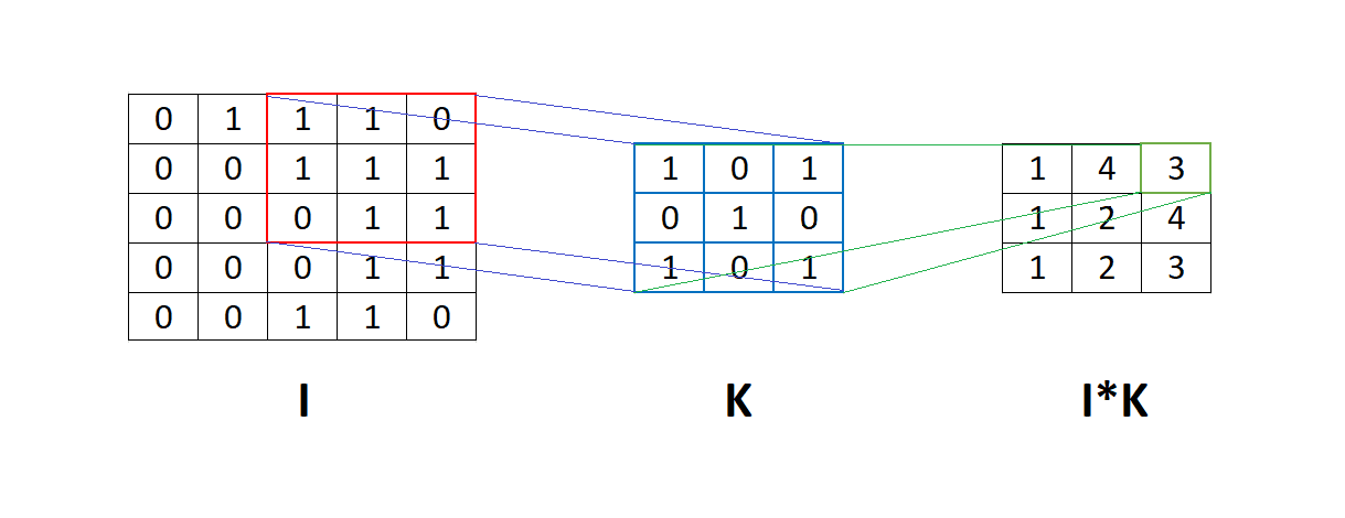
Generally, there is no significant difference in activation functions in CNN.
Theoretically, we can use every function we mentioned for FCNN, but in practice, the most common choice is to use ReLU or hyperbolic tangent. This is because the ReLU function adds additional non-linearity to the network and improves it by speeding up training. Although ReLU might cause some issues such as “dead neurons”, some modifications such as Leaky ReLU or ELU can solve that.
Convolutional neural networks have a wide range of applications, but mostly, they solve problems related to computer vision, such as image classification and object detection. Some of the key examples of CNN applications are:
This article explained the main differences between convolutional and regular neural networks. To conclude, the main difference is that CNN uses convolution operation to process the data, which has some benefits for working with images. In that way, CNNs reduce the number of parameters in the network. Also, convolution layers consider the context in the local neighborhood of the input data and construct features from that neighborhood.
For instance, pixels in the neighborhood of an image, frames in a video, words in a text, and similar.