

Learn through the super-clean Baeldung Pro experience:
>> Membership and Baeldung Pro.
No ads, dark-mode and 6 months free of IntelliJ Idea Ultimate to start with.
Learn through the super-clean Baeldung Pro experience:
>> Membership and Baeldung Pro.
No ads, dark-mode and 6 months free of IntelliJ Idea Ultimate to start with.
In this tutorial, we’ll talk about the Deep Belief Network (DBN), a generative graphical model composed of a deep structure. Mainly, we’ll walk through DBN’s, Boltzmann (BM), and Restricted Boltzmann Machine’s (RBM) architectures, and we will analyze the different approaches of a Neural Network and a DBN. We’ll also introduce the learning phase of a DBN, analyze its benefits and limitations, and mention the most common applications of DBNs and RBMs.
BM, categorized as an unsupervised algorithm, is a generative neural network first introduced by Hinton and Sejnowski in 1983. The neural network’s name comes from the fact that the Boltzman probabilistic distribution is used. In general, a BM is composed of a set of visible and hidden layers, where each visible node of a visible layer is connected with each hidden node of the hidden layer. The outputs of the nodes of the visible layers are driven as input to each node of the hidden layer. Thus a symmetric probabilistic graphical model (PGM) is formed.
Thus, in the PGM of a BM exist links between nodes of the same layer (visible or hidden) and different layers.
The difference between a BM and an RBM lies in the fact that the second network contains fewer connections than the first one. In an RBM, there are no connections between nodes of the same layer. Therefore a node of the visible/hidden layer isn’t connected with a node of the visible/hidden layer. This noticeable difference can be seen more easily in the diagram below, in which we can see the structures of a BM (a) and RBM (b):
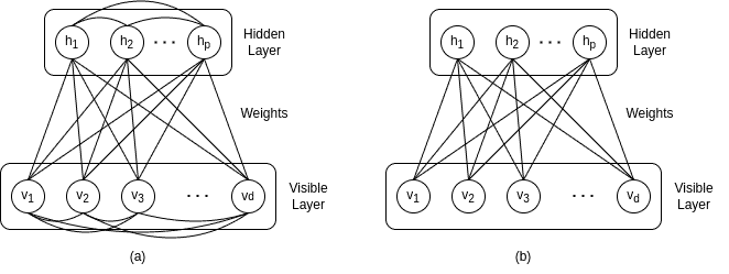
 and
and  denote the number of nodes in the hidden and visible layers, respectively.
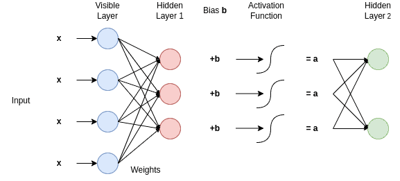
The task of an RBM is to detect patterns and inherent information by learning a probabilistic distribution. To do so, the visible layers receive the input data (for example, an image) that has to be learned. The hidden layers aim to extract useful information about the features of the data for the visible layers. The output of a node of a visible layer is multiplied with a weight  and then fed into a node of a hidden layer. Therefore, two consecutive layers form a weight matrix.
In addition, as shown in the diagram below, a bias  is added to each output of the hidden layer and then passes through an activation function. Also, the next hidden receives the inputs of the previous and acts accordingly for every single layer of the RBM network:
The training of an RBM looks into updating the weights of the links between the different layers so that the links are able to recreate the visible and hidden units as well.
A DBN is a deep-learning architecture introduced by Geoffrey Hinton in 2006. In general, a DBN architecture is considered to be a stack of RBMs. For each single RBM of the whole stack, the output of a sole RBM network is received as input from the consecutive RBM.
RBM training is a widely used technique in which several RBM architectures are stacked and used to initialize effectively a neural network. This seemed to be a very useful technique because, until that point, the random initialization of the network’s weights was insufficient and caused the vanishing gradient descent and local minima problem.
The DBN’s structure:
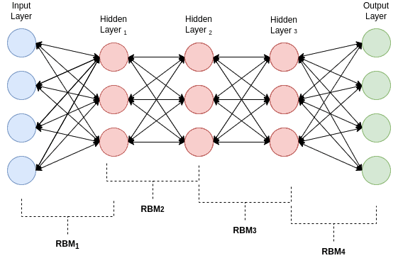
In the DBN’s architecture, two successive layers are considered to be an RBM. Regarding the RBM’s idea, the hidden units of a DBN are responsible for identifying patterns of the input’s relationships. Similarly, an intermediate matrix consists of the weights of two successive layers.
The training of a DBN is accomplished in a similar generalized manner as the RBM’s training process and follows a greedy yet effective approach. While training, the algorithm takes into account every two layers of the network, considering them to be a single RBM. The weights and biases of a single RBM are trained, and after this procedure, hidden variables are generated. These hidden variables are considered to be the visible variables of the next RBM network. The whole training phase of the DBN is considered to be finished when all the RBM stacks are trained.
Note that the first RBM (two first consecutive layers) of the DBN considers the training dataset as its visible unit.
Neural Networks and DBNs are different by definition, as the DBN is a generative probabilistic model. A DBN includes undirected interconnections between its layers (RBM connections).
Furthermore, DBNs are trained by producing the latent input features at the current layer by using the generated ones of the previous layer. On the contrary, CNN’s training focuses on learning the appropriate weights of the network by using Gradient Backward propagation.
In terms of performance, several studies have shown that CNNs seem to have better throughput and accuracy than DBNs in machine-learning tasks.
DBNs are able to manage a lot of data due to their robustness and usage of the hidden layers that assemble useful correlations of the data and can handle a wide variety of data types.
On the other hand, some of the downsides are that DBN requires a lot of data in order to achieve a decent performance at a standard level of hardware due to the size of the network, and its training is proven to be quite expensive.
The constant need for network training has highlighted the need for new data. In this case, RBMs come to contribute to the generation of new synthetic data. Also, an RBM is widely used in tasks such as dimensionality reduction, classification, regression, and feature learning.
DBNs also are used in a variety of supervised and unsupervised tasks, such as Image Classification, Object Detection, Semantic Segmentation, and Instance Segmentation. Some real-world needs and applications that include the above tasks are autonomous driving, medical image or satellite image analysis, and face recognition.
In this article, we walked through Deep Belief Networks. In particular, we mainly covered the RBM and DBN and discussed in detail their architecture and structure. Also, we discussed the learning procedure of an RMB and a DBN and mentioned the main differences between a DBN and CNN. We talked about the basic benefits and limitations of DBN. Finally, we introduced various computer vision tasks and applications that an RBM and BDN can be used.