Introduction to jVector

1. Introduction

In the fields of Artificial Intelligence and Information Retrieval, it’s common to need to search for similar vectors in a dataset. Many systems, such as recommendation systems, sentiment analysis of texts, or text generation, use vector search in their favor.

In this article, we’ll explore the jVector library for efficient index construction from datasets and vector search.

2. Understanding Vector Search

In the context of information retrieval, we can represent words as vectors, where each position represents a factor. Those factors represent the likelihood of a chosen parameter and the vectorized word. For instance, the word apple could be vectorized as [0.98, 0.2] using (‘fruit’, ‘blue’) set of parameters, because an apple is likely a fruit and it is unlikely blue.

In a system like that, we can find similar words to apple by using distance functions. For instance, the word banana could be represented as [0.94, 0.1]. Depending on the distance function, the words apple and banana are similar as they have both parameters close.

All of this boils down to the essence of vector search, which is creating a mechanism to find similar vectors with high confidence and efficiency.

3. Brief Introduction to jVector Core Structure

The vector search problem for higher-dimensional problems and big datasets is a challenge for classical vector search algorithms, due to the curse of dimensionality. Thus, to be an efficient and scalable vector search processor, jVector uses two modern structures: the Hierarchical Navigable Small Word (HNSW) graph and the Disk Approximate K-Nearest Neighbors (DiskANN) algorithm.

The HNSW is a graph structure that optimizes search by skipping unwanted vectors in the search space by using layers (or hierarchies) and links between those layers:

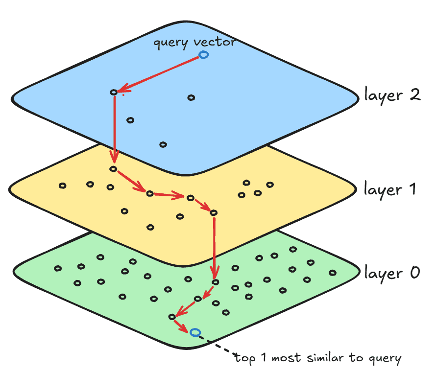
The layer 0 contains all vectors in the search space, and this is where the final search result resides. The layer 1 contains a small subset of layer 0, with more clustered vectors than layer 0. Finally, layer 2 contains a subset of layer 1, and even fewer and more clustered vectors than all other layers. The number of layers depends on the number of vectors in the search space and the graph’s degree. Those layers are built during the index structure construction that we’ll see in the following sections.

For each layer, jVector executes an instance of the DiskANN algorithm to search for similar vectors within that layer. Additionally, HNSW creates long links that connect the same vector in two different layers. Thus, when DiskANN is done processing layer 2, that is, when a local minimum is found, then the search is restarted from that same vector (using the long link between layers) in the next layer until it reaches layer 0. Finally, when DiskANN is done in the bottom-most layer, the search is done.

4. Basic Configuration

The only step needed to build jVector is to add the jVector Maven dependency:

<dependency>
    <groupId>io.github.jbellis</groupId>
    <artifactId>jvector</artifactId>
    <version>4.0.0-rc.2</version>
</dependency>

5. Graph-Based Index in jVector

In this section, we’ll learn how to build an HNSW index structure and persist it on disk.

5.1. Creating the Index

Let’s define a method to persist an index using the previously loaded vectors and a file path:

public static void persistIndex(List<VectorFloat<?>> baseVectors, Path indexPath) throws IOException {
    int originalDimension = baseVectors.get(0)
        .length();
    RandomAccessVectorValues vectorValues = new ListRandomAccessVectorValues(baseVectors, originalDimension);
    BuildScoreProvider scoreProvider = 
      BuildScoreProvider.randomAccessScoreProvider(vectorValues, VectorSimilarityFunction.EUCLIDEAN);

    try (GraphIndexBuilder builder = 
     new GraphIndexBuilder(scoreProvider, vectorValues.dimension(), 16, 100, 1.2f, 1.2f, true)) {
        OnHeapGraphIndex index = builder.build(vectorValues);
        OnDiskGraphIndex.write(index, vectorValues, indexPath);
    }
}

We first get the number of dimensions of our dataset and store the dimensions in RandomAccessVectorValues, which is essentially an efficient wrapper for a list of vector values.

We then define a BuildScoreProvider that serves as the basis for calculating distance. In the example, we’re using the Euclidean distance calculator available in the VectorSimilarityFunction class.

Then, we open up an AutoCloseable resource from the GraphIndexBuilder class using try-with-resources. Some of its parameters have an impact on how the index is built, directly affecting the quality and speed of vector search, so let’s look at each of them in order:

• scoreProvider: the score provider function
• dimension: the vector’s number of dimensions
• M: the graph’s maximum degree; naturally, more layers will be built if we set this value low
• beamWidth: the size of the beam search when DiskANN processes top-K nearest neighbors
• neighborOverflow: defines that the graph’s maximum degree can overflow by this factor temporarily during construction; must be bigger than 1
• alpha: a DiskANN parameter to control diversity of solutions; must be positive
• addHierarchy: sets whether the HNSW structure should have layers or not

Then, we call build() to build the HNSW structure based on the builder and the dataset. Finally, we write the index in a file path provided as an argument to our persistIndex() method.

5.2. Testing Index Creation

Let’s use a simple JUnit test to illustrate how client code can use our persistIndex() method:

class VectorSearchTest {
    private static Path indexPath;
    private static Map<String, VectorFloat<?>> datasetMap;

    @BeforeAll
    static void setup() throws IOException {
        datasetVectors = new VectorSearchTest().loadGlove6B50dDataSet(1000);
        indexPath = Files.createTempFile("sample", ".inline");
        persistIndex(new ArrayList<>(datasetVectors.values()), indexPath);
    }

    @Test
    void givenLoadedDataset_whenPersistingIndex_thenPersistIndexInDisk() throws IOException {
        try (ReaderSupplier readerSupplier = ReaderSupplierFactory.open(indexPath)) {
            GraphIndex index = OnDiskGraphIndex.load(readerSupplier);
            assertInstanceOf(OnDiskGraphIndex.class, index);
        }
    }
}

We first use a loadGlove6B50dDataSet() helper method to load the dataset into a map of words to their vector representation, named datasetMap. Further, we create a Path to store the output of the index and pass both the vectors and the path to our persistIndex() method. Thus, after execution of the @BeforeAll annotated method, we have the index containing the HNSW structure on disk.

Finally, we open up a ReaderSupplier to read the index on disk, and then store it as an object using load(). With all that, we can verify that the index was persisted and appropriately loaded using the desired path.

6. Searching Similar Vectors

In this section, we’ll see how to search for similar vectors using the disk index created.

To illustrate vector search, let’s add a new test method to the previously created test class with the index already loaded into disk:

@Test
void givenLoadedDataset_whenSearchingSimilarVectors_thenReturnValidSearchResult() throws IOException {
    VectorFloat<?> queryVector = datasetVectors.get("said");
    ArrayList <VectorFloat<?> vectorsList = new ArrayList<>(datasetVectors.values());

    try (ReaderSupplier readerSupplier = ReaderSupplierFactory.open(indexPath)) {
        GraphIndex index = OnDiskGraphIndex.load(readerSupplier);

        SearchResult result = GraphSearcher.search(queryVector, 10,
            new ListRandomAccessVectorValues(vectorsList, vectorsList.get(0).length()),
            VectorSimilarityFunction.EUCLIDEAN, index, Bits.ALL);

        assertNotNull(result.getNodes());
        assertEquals(10, result.getNodes().length);
    }
}

We start by defining the queryVector that we want to search for similar words. We can pick the vector representation of a word that we’ve populated previously in our datasetMap.

Then, we open up the index resource that we persisted on disk and load it into the variable index.

After that, we use the search() method present in GraphSearch to produce the similarity search result. That method accepts several parameters, so let’s look at each of them individually:

• queryVector: the query vector
• topK: the number of top similar vectors we want
• vectors: the vectors in the dataset, wrapped in ListRandomAccessVectorValues format
• similarityFunction: the vector distance calculator function
• graph: the index created previously
• acceptOrds: a variable that gives some control over which vectors are acceptable solutions; setting this to Bits.ALL says that any node in the graph is acceptable

After executing the search, we end up with a SearchResult object, containing the search result vectors. In our case, it’s ten vectors since we passed 10 as the topK.

Additionally, the result variable also contains some metadata information about the search, like how many nodes it visited.

7. Conclusion

In this article, we’ve glanced at the jVector core functionalities to build an index and search for vectors. We’ve also looked at how the HNSW and DiskANN structures work in jVector to ensure efficiency and correctness.