

Learn through the super-clean Baeldung Pro experience:
>> Membership and Baeldung Pro.
No ads, dark-mode and 6 months free of IntelliJ Idea Ultimate to start with.
Learn through the super-clean Baeldung Pro experience:
>> Membership and Baeldung Pro.
No ads, dark-mode and 6 months free of IntelliJ Idea Ultimate to start with.
In this tutorial, we’ll go over the definition of the Beam Search algorithm, explain how it works, and zoom in on the role of the beam size in the algorithm.
Beam Search is a greedy search algorithm similar to Breadth-First Search (BFS) and Best First Search (BeFS). In fact, we’ll see that the two algorithms are special cases of the beam search.
Let’s assume that we have a Graph ( ) that we want to traverse to reach a specific node. We start with the root node. The first step is to expand this node with all the possible nodes. Then, at each step of the algorithm, we choose a specific number of nodes, say
  , from the possible ones to expand. Let’s call the beam width. These nodes are the optimal ones based on our heuristic cost. The expansion continues until reaching the goal node.
Let’s keep in mind that if  , it’ll become BeFS algorithm since we’ll select the best one to expand at each step which is exactly how BeFS works. But, on the other hand, if
  , it becomes the breadth-first search. The reason is that, when selecting the nodes to expand, we’ll consider all the possible ones that are reachable from the current node with one move and without any criteria.
Assuming that we want to perform beam search on a graph, here’s its pseudocode:
algorithm BeamSearch(G, s, g, β):
    // INPUT
    //    G = the graph to search
    //    s = the start node
    //    g = the goal node
    //    beta = the beam width
    // OUTPUT
    //    the path with the lowest cost

    openList <- {s}
    closedList <- an empty list
    path <- an empty list

    while openList is not empty:
        b <- best node from openList

        openList.remove(b)
        closedList.add(b)

        if b is g:
            path.add(b)
            return path

        N <- neighbors(b)

        for n in N:
            if n is in neither closedList nor openList:
                openList.add(n)
            else if n is in openList:
                if path with current parent <= path with old parent:
                    Replace parents of n
            else if n is not in closedList:
                openList.add(n)

        if number of nodes in openList > beta:
            openList <- best beta nodes in openList

return pathA widely adopted application of beam search is in encoder-decoder models such as machine translation. When translating one language to another, we first encode a sequence of words from the source language and then decode the intermediate representation into a sequence of words in the target language. In the decoding process, for each word in the sequence, there can be several options. This is where the beam search comes into play.
Let’s go through a simplified sample decoding process step by step. In this example, our heuristic function will be the probability of words and phrases that are possible in translation. First, we start with a token that signals the beginning of a sequence. Then, we can obtain the first word by calculating the probability of all the words in our vocabulary set. We choose  (beam width) words with highest probabilities as our initial words (
 ):
):
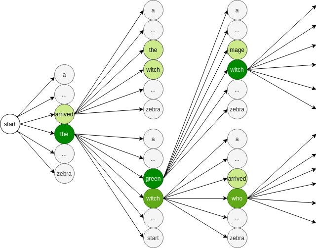
After that, we expand the two words and compute the probability of other words that can come after them. The words with the highest probabilities will be  . From these possible paths, we choose the two most probable ones (
 ). Now we expand these two and get other possible combinations (
 ). Once again, we select two words that maximize the probability of the current sequence (
 ). We continue doing this until we reach the end of the sequence. In the end, we’re likely to get the most probable translation sequence.
We should keep in mind that along the way, by choosing a small , we’re ignoring some paths that might have been more likely due to long-term dependencies in natural languages. One way to deal with this problem is to opt for a larger beam width.
Compared to best-first search, an advantage of the beam search is that it requires less memory. This is because it doesn’t have to store all the successive nodes in a queue. Instead, it selects only the best (beam width) ones.
On the other hand, it still has some of the problems of BeFS. The first one is that it is not complete, meaning that it might not find a solution at all. The second problem is that it is not optimal either. Therefore, when it returns a solution, it might not be the best solution.
The beam width is the hyperparameter of the beam search. The selection of this hyperparameter depends on the application we are working on and how accurate we want it to be. For instance, in our example above, a larger beam width can help to choose the words that make more accurate long phrases. However, the downside of a larger beam width is that it’ll require more memory.
Overall, larger beam widths result in better solutions at the cost of more memory. Therefore, we should strike a balance between the two based on the available resources.
In this article, we learned about the Beam Search algorithm, its pros and cons, and the role of the beam size as a hyperparameter.