Time and Space Complexity of Adjacency Matrix and List

1. Overview

In this tutorial, we’ll learn one of the main aspects of Graph Theory — graph representation. The two main methods to store a graph in memory are adjacency matrix and adjacency list representation. These methods have different time and space complexities.

Thus, to optimize any graph algorithm, we should know which graph representation to choose. The choice depends on the particular graph problem. In this article, we’ll use Big-O notation to describe the time and space complexity of methods that represent a graph.

2. Graph Representation

It’s important to remember that the graph is a set of vertices $V$ that are connected by edges $E$ . An edge is a pair of vertices $e_{ij} = (v_{i}, v_{j})$ , where $v_{i}, v_{j} \subset V$ . Each edge has its starting and ending vertices. If graph is undirected, $e_{ij} = (v_{i}, v_{j}) = (v_{j}, v_{i}) = e_{ji}$ . But, in directed graph the order of starting and ending vertices matters and $e_{ij} \neq e_{ji}$ .

Here is an example of an undirected graph, which we’ll use in further examples:

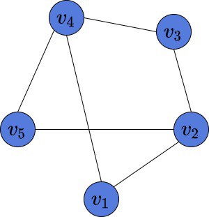
This graph consists of 5 vertices $v_{1}, v_{2}, v_{3}, v_{4}, v_{5}$ , which are connected by 6 edges $(v_{1}, v_{2}), (v_{1}, v_{4}), (v_{2}, v_{3}), (v_{2}, v_{5}), (v_{3}, v_{4})$ , and $(v_{4}, v_{5})$ .

Some graphs might have many vertices, but few edges. These ones are called sparse. On the other hand, the ones with many edges are called dense. Our graph is neither sparse nor dense. However, in this article, we’ll see that the graph structure is relevant for choosing the way to represent it in memory.

3. Adjacency Matrix

The first way to represent a graph in a computer’s memory is to build an adjacency matrix. Assume our graph consists of $n$ vertices numbered from $1$ to $n$ . An adjacency matrix is a binary matrix of size $n \times n$ . There are two possible values in each cell of the matrix: 0 and 1. Suppose there exists an edge between vertices $v_{i}$ and $v_{j}$ . It means, that the value in the $i^{th}$ row and $j^{th}$ column of such matrix is equal to 1. Importantly, if the graph is undirected then the matrix is symmetric.

3.1. Example

Here is an example of an adjacency matrix, corresponding to the above graph:

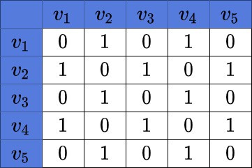
We may notice the symmetry of the matrix. Also, we can see, there are 6 edges in the matrix. It means, there are 12 cells in its adjacency matrix with a value of 1.

3.2. Time and Space Complexity

Assuming the graph has $\boldsymbol{n}$ vertices, the time complexity to build such a matrix is $\boldsymbol{O(n^2)}$ . The space complexity is also $\boldsymbol{O(n^2)}$ . Given a graph, to build the adjacency matrix, we need to create a square $n \times n$ matrix and fill its values with 0 and 1. It costs us $O(n^2)$ space.

To fill every value of the matrix we need to check if there is an edge between every pair $(v_{i}, v_{j})$ of vertices. The amount of such pairs of $n$ given vertices is ${n \choose 2} = \frac{n \times (n - 1)}{2}$ . That is why the time complexity of building the matrix is $O(n^2)$ .

3.3. Pros and Cons

The advantage of such representation is that we can check in $\boldsymbol{O(1)}$ time if there exists edge $\boldsymbol{e_{ij} = (v_{i}, v_{j})}$ by simply checking the value at $\boldsymbol{i^{th}}$ row and $\boldsymbol{j^{th}}$ column of our matrix.

However, this approach has one big disadvantage. We need $O(n^2)$ space in the only case — if our graph is complete and has all ${n \choose 2} = \frac{n \times (n - 1)}{2}$ edges. The matrix will be full of ones except the main diagonal, where all the values will be equal to zero. But, the complete graphs rarely happens in real-life problems. So, if the target graph would contain many vertices and few edges, then representing it with the adjacency matrix is inefficient.

4. Adjacency List

The other way to represent a graph in memory is by building the adjacent list. If the graph consists of $n$ vertices, then the list $L$ contains $n$ elements. Each element $L_{i}$ is also a list and contains all the vertices, adjacent to the current vertex $v_{i}$ . By choosing an adjacency list as a way to store the graph in memory, this may save us space.

For instance, in the Depth-First Search algorithm, there is no need to store the adjacency matrix. At each algorithm step, we need to know all the vertices adjacent to the current one. This what the adjacency lists can provide us easily. We may also use the adjacency matrix in this algorithm, but there is no need to do it. Instead, we are saving space by choosing the adjacency list.

4.1. Example

This is the adjacency list of the graph above:

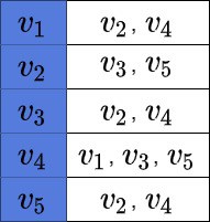
We may notice, that this graph representation contains only the information about the edges, which are present in the graph.

4.2. Time and Space Complexity

If $\boldsymbol{m}$ is the number of edges in a graph, then the time complexity of building such a list is $\boldsymbol{O(m)}$ . The space complexity is $\boldsymbol{O(n + m)}$ . But, in the worst case of a complete graph, which contains ${n \choose 2}$ edges, the time and space complexities reduce to $O(n^2)$ .

4.3. Pros and Cons

As it was mentioned, complete graphs are rarely meet. Thus, this representation is more efficient if space matters. Moreover, we may notice, that the amount of edges doesn’t play any role in the space complexity of the adjacency matrix, which is fixed. But, the fewer edges we have in our graph the less space it takes to build an adjacency list.

However, there is a major disadvantage of representing the graph with the adjacency list. The access time to check whether edge $e_{ij} = (v_{i}, v_{j})$ is present is constant in adjacency matrix, but is linear in adjacency list. In a complete graph with $n$ vertices, for every vertex $v_{i}$ the element of $L_{i}$ would contain $n - 1$ element, as every vertex is connected with every other vertex in such a graph.

Therefore, the time complexity checking the presence of an edge in the adjacency list is $\boldsymbol{O(n)}$ . Let’s assume that an algorithm often requires checking the presence of an arbitrary edge in a graph. Also, time matters to us. Here, using an adjacency list would be inefficient.

5. Removing Edges and Vertices

Let’s now see the worst-case complexity of removing a vertex and an edge.

5.1. Removing a Vertex

Let’s suppose we want to remove $v_i$ .

If we use the adjacency matrix, we’ll have to set all the entries in the $i$ -th row and the $i$ -th column to zero. Doing so will delete all the edges incident to $v_i$ , effectively removing $v_i$ from the graph. In total, we’ll iterate over $2n$ cells, so the time complexity will be $\boldsymbol{O(n)}$ .

On the other hand, removing a vertex from an adjacency list will cost more. To remove all the outgoing edges, we set to NULL the pointer to the $v_i$ ‘s list, $L_i$ . However, to delete all the occurrences of $v_i$ from other nodes’ lists, we have to iterate over all the other lists. In the worst case, each node will be connected to all the other vertices, so we’ll traverse $(n-1)n$ list elements. Therefore, removing a vertex from the list representation of a graph is an $\boldsymbol{O(n^2)}$ operation.

5.2. Removing an Edge

To remove an edge $e_{ij}$ from an adjacency matrix $M$ , we set $M[i,j]$ to zero. If the graph is symmetric, we do the same with $M[j, i]$ . Accessing a cell in the matrix is an $\boldsymbol{O(1)}$ operation, so the complexity is $\boldsymbol{O(1)}$ in the best-case, average-case, and worst-case scenarios.

If we store the graph as an adjacency list, the complexity of deleting an edge is $\boldsymbol{O(n)}$ . That’s because, in the worst case, we traverse the whole list $L_i$ to remove $v_j$ from it. If the graph is symmetric, we do the same with $L_j$ , removing $v_i$ from it. In total, we iterate over no more than $2n$ elements, so the complexity is $O(n)$ .

6. Conclusion

In this tutorial, we’ve discussed the two main methods of graph representation. We’ve learned about the time and space complexities of both methods. Moreover, we’ve shown the advantages and disadvantages of both methods.

The choice of the graph representation depends on the given graph and given problem. In some problems space matters, however, in others not. These assumptions help to choose the proper variant of graph representation for particular problems.

Full Archive

About Baeldung

Core Concepts

Operating Systems

Artificial Intelligence

Graph Theory

Latex