

Learn through the super-clean Baeldung Pro experience:
>> Membership and Baeldung Pro.
No ads, dark-mode and 6 months free of IntelliJ Idea Ultimate to start with.
Last updated: February 28, 2025
Learn through the super-clean Baeldung Pro experience:
>> Membership and Baeldung Pro.
No ads, dark-mode and 6 months free of IntelliJ Idea Ultimate to start with.
In this tutorial, we’ll walk through two approaches used for decision-making in dynamic systems, Reinforcement Learning (RL) and optimal control. We’ll introduce the two types and analyze their main differences and usages.
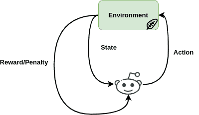
In machine learning, RL learning trains certain agents by making them make decisions about a certain concept. Then, based on the decision they make, they either are rewarded or face the consequences with a penalty that has been defined.
So these agents make decisions in a specific environment about a problem, take action and then receive feedback to improve their decisions on their next move and maximize their cumulative reward. Therefore, RL is a trial-and-error interactive game, where agents aim to learn a policy, behave according to it, and try to find the optimal solution to this policy depending on their actions:
An MDP is defined by a set of states  , a set of actions
  , and a transition function
  that defines the probability of transitioning to a new state
  when taking action
  in state
  . It also includes a reward function
  that gives the reward for taking action in state .
The value function  is defined as the expected cumulative reward starting from state s and following the policy
  :
:
(1) ![\begin{equation*}\begin{aligned} V_{\pi}(s) = \mathbb{E}[R(s, \pi(s)) + \gamma \cdot \sum s'\in S \cdot T(s'|s, π(s)) \cdot V_{\pi}(s')] \end{aligned} \end{equation*}](/wp-content/ql-cache/quicklatex.com-25ab36fc1b52374b10cd3c92a2ebaf5a_l3.svg "Rendered by QuickLaTeX.com")
where  is the discount factor that controls the trade-off between immediate and future rewards.
The goal of the RL agent is to find the optimal policy that maximizes the value function .
Several algorithms can be used to find the optimal policy. These algorithms differ in how they estimate the value function and update the policy. RL algorithms can be divided into three main categories: value-based methods, policy-based methods, and model-based methods.
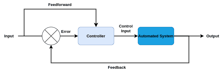
On the other hand, optimal control is mainly used in physics and engineering system design and focuses on the efficiency of a system.
Its goal is to model the best strategy for a certain system in a fixed period of time in an optimal way. Typically, this strategy is about minimizing a mathematical cost function, which usually is about the performance of the system.
Therefore the whole system is modeled by mathematical equations that describe the system’s behavior. Usually, these equations consider the input, output, time, and general cost function, along with known specific constraints. The block diagram below helps in understanding the optimal control’s basic concept:
DP is helpful where the number of states is limited and the dynamics are known. It divides an optimal control issue into smaller subproblems and recursively solves each.
PMP, another optimal control method, employs the Hamiltonian of the system to find the optimal control input. Problems involving continuous states and control inputs benefit most from it.
Another optimal control algorithm is the HJB equation which uses partial differential equations to find the value function of the system. HJB is also useful for problems with continuous states and control inputs.
Both RL and optimal control focus on making optimal decisions in dynamic systems but have slight differences in the way they deal with the problem.
First of all, RL employs agents that learn a certain policy that links states to actions in an attempt to increase their total reward through time. In case these agents make bad decisions, they receive penalties.
On the other hand, optimal control is more mathematically straightforward as it aims at finding an optimal input that minimizes a cost function. Moreover, in optimal control, the initial, final, and cost functions are known.
Both RL and optimal control are applied in different real-world applications and tasks. RL is mostly employed in the fields of robotics and gaming. In robotics, RL has been used to train robots to perform tasks. In gaming, RL has been used to train agents to play games like chess.
Optimal control is used in aerospace, automotive, and power systems. In aerospace and automotive optimal control is used in the design of control systems and guidance. Additionally, designing control systems for power stations and electric grids have also been employed in power systems.
In this tutorial, we walked through RL and optimal control. In particular, we introduced these two methods, discussed their mathematical approaches, and highlighted their main differences and applications.