Markov Decision Process: How Does Value Iteration Work?

1. Introduction

In some machine learning applications, we’re interested in defining a sequence of steps to solve our problem. Let’s consider the example of a robot trying to find the maze exit with several obstacles and walls.

The focus of our model should be how to classify a whole sequence of actions from the initial state that brings the robot to the desired state outside of the maze.

In Machine Learning, this type of problem is usually addressed by the Reinforcement Learning (RL) subfield that takes advantage of the Markov decision process to model part of its architecture. One of the challenges of RL is to find an optimal policy to solve our task.

In this tutorial, we’ll focus on the basics of Markov Models to finally explain why it makes sense to use an algorithm called Value Iteration to find this optimal solution.

2. Markov Models

To model the dependency that exists between our samples, we use Markov Models. In this case, the input of our model will be sequences of actions that are generated by a parametric random process.

In this article, our notation will consider that a system with $N$ possible states $S_{1},S_{2},...,S_{N}$ will be at a time $t=1,2,...$ in a state $q_{t}$ . So, the equality $q_{3}=S_{2}$ indicates that at the time $3$ , the system will be at the state $S_{2}$ .

We should highlight that the subscript $t$ is referred to as time, but it could be other dimensions, such as space.

But how can we put together the relationship between all possible states in our system? The answer is to apply the Markov Modelling strategy.

2.1. Theoretical Fundamentals

If we are at a state $S_{i}$ at the time $t$ , we can go to state $S_{j}$ at the time $t+1$ with a given or calculated probability that depends on previous states:

(1) $\begin{equation*} P(q_{t+1}=S_{j}|q_{t}=S_{i}, q_{t-1}=S_{k},...) \end{equation*}$

To make our model slightly simpler, we can consider that only the immediately previous state influences the next state instead of all preceding states. Only the current state is relevant to define the future state, and we have a first-order Markov model:

(2) $\begin{equation*} $P(q_{t+1}=S_{j}|q_{t}=S_{i})$ \end{equation*}$

To simplify our model a little more we remove the time dependency and we define that from a state $S_{i}$ we’ll go to a state $S_{j}$ by the means of a transition probability:

(3) $\begin{equation*} a_{i,j} = P(q_{t+1}=S_{j}|q_{t}=S_{i}) \end{equation*}$

One of the easiest ways for us to understand these concepts is to visualize a Markov Model with two states connected by four transitions:

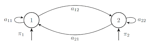
The variable $\pi_{i}$ represents the probability of starting at state $i$ . As we removed the time dependency from our model, at any moment, the transition probability of going from state $1$ to $2$ will be equal to $a_{12}$ regardless of the value of $t$ .

Moreover, the transition probabilities for a given state $S_{i}$ should satisfy one condition:

(4) $\begin{equation*} \sum_{j=1}^{N}a_{ij}=1 \end{equation*}$

For the $\pi_{i}$ case we have an equivalent condition, since the sum of all possible initial states should be equal to $100\%$ :

(5) $\begin{equation*} \sum_{i=1}^{N}\pi_{i}=1 \end{equation*}$

Lastly, if we know all states $q_{t}$ , our output will be the sequence of the states from an initial to a final state, and we’ll call this sequence observation sequence $O$ . The probability of a sequence can be calculated:

(6) $\begin{equation*} P(O=Q|\boldsymbol{A,\Pi}) = P(q_{1}) \prod_{t=2}^{T}P(q_{t}|q_{t-1})=\pi_{q_{1}}a_{q_{1}q_{2}}...a_{q_{T-1}q_{T}} \end{equation*}$

In which $\boldsymbol{\Pi}$ represents the sum of initial probabilities and $\boldsymbol{A}$ is the vector of transition probabilities. $\pi_{q_{1}}$ represents the probability of start at state $q_{1}$ . While $a_{q_{1}q_{2}}$ represents the probability of reach state $q_{2}$ from $q_{1}$ .

To illustrate all this theory, let’s consider $\pi_{1}=0.7$ and $\pi_{2}=0.3$ with defined values for the transition probabilities:

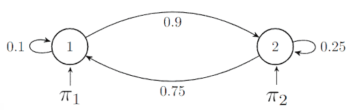
We’ll consider the observation sequence $O = \{1, 2, 2\}$ . The probability of this sequence can be calculated:

(7) $\begin{equation*} P(O=Q|\boldsymbol{A,\Pi}) = P(q_{1}) \cdot P(q_{2}|q_{1}) \cdot P(q_{2}|q_{2}) \end{equation*}$

After we replace the defined values:

(8) $\begin{equation*} = \pi_{1} \cdot a_{12} \cdot a_{22} = 0.7 \cdot 0.9 \cdot 0,25 = 0.1575 \end{equation*}$

2.2. Hidden Markov Models

In the previous example, all states were known, so we call them observable. When the states are not observable, we have a hidden Markov model (HMM).

To define the probabilities of a state, we first need to visit this state and then write down the probability of the observation. We consider a good HMM model one that correctly uses real-world data to create a model to simulate the source.

It is crucial that we remember that in this type of model, we have two sources of randomness: the observation in a state and the movement from one state to another.

We usually have two main problems in HMM:

Considering a model $\lambda$ , we’re interested in calculating the probability $P(O|\lambda)$ , which means the probability of any observation sequence $O$
Finding the state sequence with the higher chances of generating the observation sequence $O$

3. Reinforcement Learning

As we stated in the introduction of this article, some problems in Machine Learning should have as a solution a sequence of actions instead of a numeric value or label.

In Reinforcement Learning, we have an agency responsible for the decision-making to select an action in an environment.

3.1. Example

At any given state, the agent will take an action, and the environment will return a reward or penalty. A sequence of actions is called policy, and the primary goal of an RL problem is to find the optimal policy to maximize the total reward.

If we return to the initial example of a robot trying to find the exit of a maze, the robot would be the learner agent, and the environment would be the labyrinth:

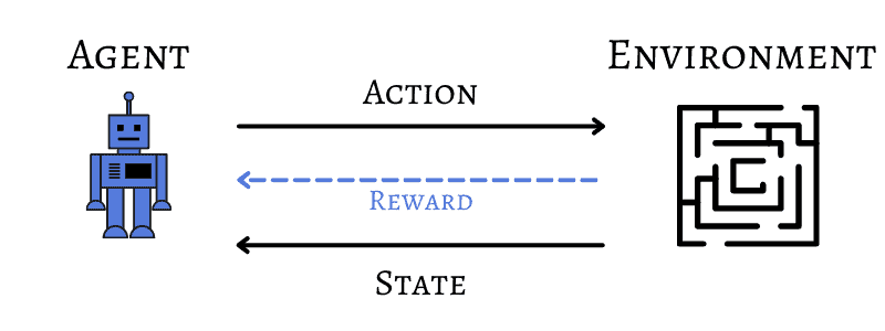
From this point, we can make an analogy with the Markov model since the solution for this problem is a sequence of actions.

A Markov Decision Process is used to model the agent, considering that the agent itself generates a series of actions. In the real world, we can have observable, hidden, or partially observed states, depending on the application.

3.2. Mathematical Model

In our explanation, we’ll consider that the agent will be at a state $s_{t}$ in a given discrete-time $t$ . The variable $S$ will represent all the possible states. The available actions will be represented as $A(s_{t})$ , and after an action is taken and the agent goes from $s_{t}$ to $s_{t+1}$ a reward $r_{t+1}$ is computed.

As we defined before, we have here a first-order Markov model since the next state and reward depend only on the current state and action.

From now on, we’ll consider that the policy $\pi$ defines the mapping of states to actions $\pi: S \to A$ . So, if we’re at a state $s_{t}$ , the policy will indicate the action to be taken.

The value of a policy referred to as $V^{\pi}(s_{t})$ is the expected value after all the rewards of a policy are summed starting from $s_{t}$ . If we put into our mathematical model:

(9) $\begin{equation*} V^{\pi}(s_{t})= E[r_{t+1}+r_{t+2}+ \ldots + r_{t+T}]= E\left[ \sum_{i=1}^{T} r_{t+1} \right] \end{equation*}$

We should highlight that the above equation only works when we have a defined number of steps $T$ to take. In case we don’t have this value, we have an infinite-horizon model that will penalize future rewards by means of a discount rate $\gamma$ :

(10) $\begin{equation*} V^{\pi}(s_{t})= E[r_{t+1}+\gammar_{t+2}+ \gamma^{2}r_{t+3} + \ldots = E\left[ \sum_{i=1}^{\infty} \gamma^{i-1}r_{t+i} \right] \end{equation*}$

Our main goal is to find the optimal policy $\pi^{*}$ that will lead our cumulative reward to its maximum value:

(11) $\begin{equation*} V^{*}(s_{t})= max \: V^{\pi}(s_{t}), \forall s_{t} \end{equation*}$

We can also use a pair of state and action to indicate the impact of taking action $a_{t}$ being at the state $s_{t}$ . We leave the use of $V(s_{t})$ to simply indicate the performance of being at state $s_{t}$ .

We start from the knowledge that the value of a state is equal to the value of the best possible action:

(12) $\begin{equation*} V^{*}(s_{t})=max \: Q^{*}(s_{t},a_{t}) \end{equation*}$

(13) $\begin{equation*} V^{*}(s_{t}) = max \left( E[r_{t+1}]+\gamma \sum_{s_{t+1}}^{} P(s_{t+1}|s_{t},a_{t})V^{*}(s_{t+1}) \right) \end{equation*}$

This represents the expected cumulative reward $V^{*}(s_{t+1})$ considering that we move with probability $P(s_{t+1}|s_{t},a_{t})$ .

If we use the state-action pair notation, we have:

(14) $\begin{equation*} Q^{*}(s_{t},a_{t})=E[r_{t+1}]+ \gamma \sum_{s_{t+1}} P(s_{t+1}|s_{t},a_{t}) max \: Q^{*}(s_{t+1},a_{t+1}) \end{equation*}$

4. Value Iteration

Finally, to find our optimal policy for a given scenario, we can use the previously defined value function and an algorithm called value iteration, which is an algorithm that guarantees the convergence of the model.

The algorithm is iterative, and it will continue to execute until the maximum difference between two consecutive iterations $l$ , and $l+1$ is less than a threshold $\delta$ :

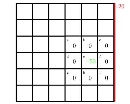
Now we’ll see a simple example of the value iteration algorithm simulating an environment.

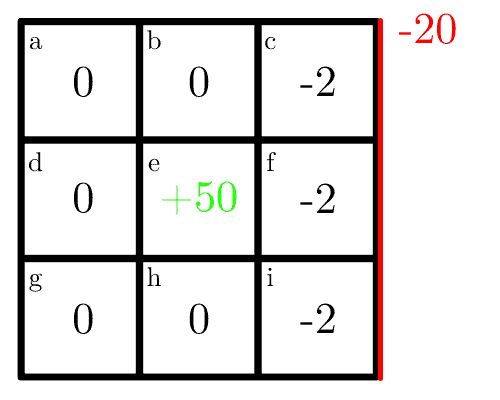
Our full map is a $6 \times 6$ grid, but for the sake of simplicity, we’ll consider a small part of the maze consisting of a $3 \times 3$ grid with a reward of $50$ in the center with their values initialized to zero.

Our robot can only take four actions: move up, down, left or right, and if it hits the wall to the right, it receives a penalty of $20$ :

As we’re simulating a stochastic model, there are probabilities associated with the actions. In this case, there is a $0.7$ chance of the robot actually going in the defined direction and a $0.1$ chance for the other three options of movement.

So if the agent decides to go top, there is a 70% chance of going top and a 10% chance of going down, right or left, each. The robot only gets the reward when the action is completed, not during the transition.

In the first iteration, each cell receives its immediate reward. As the optimal for the cell $c$ is going down with a $0.1$ probability of hitting the wall, we can calculate the immediate reward as $(0.1 \times 20)=-2$ , and the map becomes:

For the next steps, we’ll use a discount rate $\gamma = 0.9$ . For the second iteration, we’ll consider first the cell $f$ , and we’ll calculate the value of going taking the optimal action, which is going left:

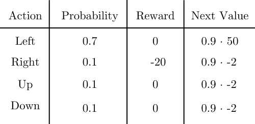
The state value will be the sum of the reward and the next value multiplied by the probability for all actions:

(15) $\begin{equation*} 0.7 (0+ (0.9 \times 50)) + 0.1(-20+(0.9 \times -2)) + 0.1(0+(0.9 \times -2)) + 0.1(0+(0.9 \times -2)) =31.5 -2.18 -0.18 -0.18 = 28.96 \end{equation*}$

Similarly, to cell $d$ we observe that the optimal action is to go right and all other directions give a expected reward of zero, so the state value is simply:

(16) $\begin{equation*} 0.7 (0 + 0.9 \times 50) = 31.5 \end{equation*}$

After we calculate for all cells, the map becomes:

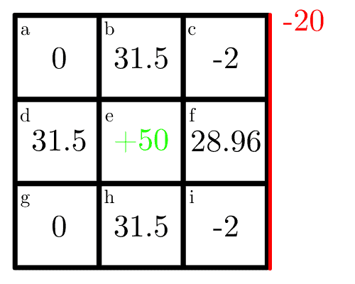
We only conducted two iterations, but the algorithm continues until the desired number of iterations of the threshold is achieved.

5. Conclusion

In this article, we discussed how we could implement a dynamic programming algorithm to find the optimal policy of an RL problem, namely the value iteration strategy.

This is an extremely relevant topic to be addressed since the task of maximizing the reward in this type of model is the core of real-world applications. Since this algorithm is guaranteed to find the optimal values and to converge, it should be considered when implementing our solution.

Full Archive

About Baeldung

Core Concepts

Operating Systems

Artificial Intelligence

Graph Theory

Latex