

Learn through the super-clean Baeldung Pro experience:
>> Membership and Baeldung Pro.
No ads, dark-mode and 6 months free of IntelliJ Idea Ultimate to start with.
Learn through the super-clean Baeldung Pro experience:
>> Membership and Baeldung Pro.
No ads, dark-mode and 6 months free of IntelliJ Idea Ultimate to start with.
In this tutorial, we’ll explain random variables.
Let’s say that  is the set of all possible outcomes of a random process we’re analyzing. We call
  the sample space. For instance, when tossing a coin, there are two outcomes: head (
 ) and tail (
 ), so
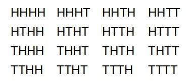
), so  . Similarly, when flipping a coin 4 times in a row, there are
  outcomes in the sample space:
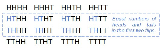
An event is any subset of . For example:
If we define a probability  telling us how likely each event is, we get a probability space. More precisely, maps the events defined over to
 ![[0, 1]](/wp-content/ql-cache/quicklatex.com-944fdd98d4f1854c8720f98d8b20b6ad_l3.svg "Rendered by QuickLaTeX.com") . That’s where random variables come into play.
. That’s where random variables come into play.
Usually, we’re interested in the numerical values the events represent or can be assigned. For example, if we toss a coin 100 times, we may be interested only in the number of heads and not the exact sequence of the s and s.
Intuitively speaking, random variables are numerical interpretations of events. Those numerical values aren’t arbitrary. They represent precisely those quantities we’re interested in.
So, a random variable  maps events to numbers
  . Using the events’ probability , we derive the probability
  with which
  takes values from .
For example, if our coin is fair, each outcome in is equally likely. If we define as the number of heads in four flips, we get this :
![\[\begin{pmatrix} 0 & 1 & 2 & 3 & 4 \\ \frac{1}{16} & \frac{1}{4} & \frac{3}{8} & \frac{1}{4} & \frac{1}{16} \end{pmatrix}\]](/wp-content/ql-cache/quicklatex.com-9fcdba20cf397332c20003612cb00a84_l3.svg "Rendered by QuickLaTeX.com")
There are two main types of random variables: discrete and continuous.
We say that is discrete if the set of values it can take with a non-zero probability is countable.
For instance, if is finite, is a discrete random variable. But, a variable can take infinitely many values and still be discrete.
Let’s say we’re flipping a coin until we get two heads in a row. We can get  in the first two flips, but there may be a sequence of 100 s before we get the first . In fact, we may never get two s one after another since there’s always a non-zero chance to get a after an .
So, if our random variable represents the number of tosses until getting two s in a row, the set of its values will be infinite:
![\[2, 3, 4, \ldots\]](/wp-content/ql-cache/quicklatex.com-762ed18db7a9bcaadd8bc3f982e6c408_l3.svg "Rendered by QuickLaTeX.com")
However, it’s still countable! That means we can arrange it as an array. Since each value is possible with a non-zero probability, we say that the is discrete.
Mathematically speaking, the probability is defined over subsets of just as the probability is defined over subsets of . The function mapping individual values  of to their probabilities is known as the probability mass function (PMF)
  .
.
The distinction is technical for the most part since we can define one using the other. Here’s how we get PMF from :
![\[p_X(x) = P_X(\{ x\}) \quad (\forall x \in \mathcal{B})\]](/wp-content/ql-cache/quicklatex.com-389d14c0829eb9e5793b24dad4d62a64_l3.svg "Rendered by QuickLaTeX.com")
and vice versa:
![\[P_X(E) = \sum_{x \in E}p_X(x) \quad (\forall E \subseteq \mathcal{B})\\\]](/wp-content/ql-cache/quicklatex.com-f7d0ab3660b311140930cbe6955d7ac6_l3.svg "Rendered by QuickLaTeX.com")
Let  be any value can take. The cumulative distribution function (CDF) of is defined as:
![\[\mathrm{CDF}_X(x) = P_X(X \leq x)\]](/wp-content/ql-cache/quicklatex.com-0fb917452aa10cdafcb77818ea53fdc5_l3.svg "Rendered by QuickLaTeX.com")
For discrete variables, we calculate the CDF by summing individual probabilities:
![\[\mathrm{CDF}_X(x) = \sum_{z \in \mathcal{B} \mid z \leq x} p_X(z)\]](/wp-content/ql-cache/quicklatex.com-e8a587491d293e827044a857ede44e55_l3.svg "Rendered by QuickLaTeX.com")
In our example with 4 tosses and with denoting the number of heads,  shows us the probability to get or fewer heads:
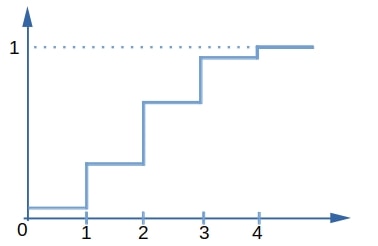
As we see, plotting  against sorted reveals a non-decreasing staircase function. The probability that gets a value between
  and
and  is the corresponding area under the CDF.
We calculate it as follows:
![\[P_X(a\leq X \leq b) = F_X(b) - F_X(a)\]](/wp-content/ql-cache/quicklatex.com-7c9d7688615c7c7c3c9f438a351ab148_l3.svg "Rendered by QuickLaTeX.com")
We differentiate between various types of variables depending on the shapes of their CDFs.
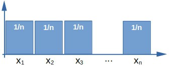
For instance, a uniform discrete variable assigns equal probabilities to each value in :
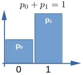
If there are only two values can take, which we usually denote as 0 and 1, we have a Bernoulli random variable:
Let model the time (in minutes) we spend waiting for an order in a restaurant. Let’s also say that the restaurant guarantees the waiting time is 15 minutes at most. So, ![X=[0, 15]](/wp-content/ql-cache/quicklatex.com-3207007cc7ca8d653e46fa3ef469a7f6_l3.svg "Rendered by QuickLaTeX.com") . In what ways is this different from the count of s discussed above?
. In what ways is this different from the count of s discussed above?
First, there are uncountably many different values it can take: 10, 11, 10.5, 10.55, 10.555 minutes, and so on. But that’s not the most important difference.
The probability  is spread over the uncountably many values in the range
 ![[0, 15]](/wp-content/ql-cache/quicklatex.com-9767beca292fd5b281ea9501fe8fbe99_l3.svg "Rendered by QuickLaTeX.com") . Since all those values are possible, we need to allocate some probability to each one. However, because there are infinitely many of them, and the total probability is finite (=1), the allocated amounts get so small that they’re practically zero (
. Since all those values are possible, we need to allocate some probability to each one. However, because there are infinitely many of them, and the total probability is finite (=1), the allocated amounts get so small that they’re practically zero ( ). So, if we single out an individual value
 ![x \in [0, 15]](/wp-content/ql-cache/quicklatex.com-61fbcf44ee6d66a03725d200c4474207_l3.svg "Rendered by QuickLaTeX.com") , the probability of its realization
, the probability of its realization  is zero.
That’s the definition of continuous variables. A random variable is continuous if  for every value
  it can take.
The CDF of a continuous random variable is continuous everywhere:
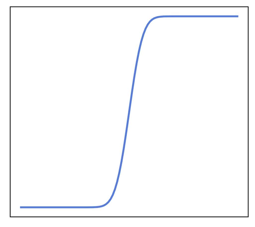
The jumps and the staircase shape of a discrete variable’s CDF happen at the points at which  . Since
  for each
  if is continuous, there can be no jumps in the CDF plot. By definition, that means the corresponding CDF is continuous.
If  has a derivative
  , it holds that:
![\[\mathrm{CDF}_X(x) = \int_{-\infty}^{x}f_X(u)du\]](/wp-content/ql-cache/quicklatex.com-128779eb92fc5489e8b23f8500787481_l3.svg "Rendered by QuickLaTeX.com")
We call such a function the probability density function (PDF) of . It’s zero outside the variable’s support, and the integral over it must be equal to 1:
![\[\int_{-\infty}{\infty}f_X(u)du = 1\]](/wp-content/ql-cache/quicklatex.com-00c655a64c7940fa60188304b97c127c_l3.svg "Rendered by QuickLaTeX.com")
Otherwise, it isn’t a proper density since we’ll get a total probability greater or lower than 100%, which doesn’t make sense.
The PDF of a continuous variable is analogous to the PMF of a discrete one. Both functions take the variable’s individual values as arguments. However, while PMF reveals their probabilities, the PDF shows us only how likely the values are one versus the other.
A continuous uniform variable’s PDF is constant over the range it’s defined over:
![\[f_X(u) = \frac{1}{b-a} \quad \text{ if } \mathcal{B} = [a, b]\]](/wp-content/ql-cache/quicklatex.com-74c5a5ed180e72e39901aaabeae767cb_l3.svg "Rendered by QuickLaTeX.com")
So the corresponding CDF is:
![\[\mathrm{CDF}_X(x) = \frac{x - a}{b - a}\]](/wp-content/ql-cache/quicklatex.com-4878fa590c9717298b6d1d2d6ce97283_l3.svg "Rendered by QuickLaTeX.com")
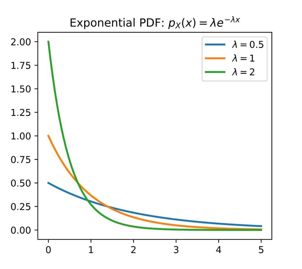
Another example is the class of exponential variables. Their densities drop exponentially, so small values are more likely than larger ones. The rate at which the density decreases is controlled by a parameter we usually denote as  :
:
Here’s a summary of the differences between discrete and continuous random variables:
| Discrete | Continuous |
|---|---|
| Countably many values with positive probabilities | No values with positive probabilities |
| Non-continuous step CDF | Continuous CDF |
| Usually denote counts | Usually represent measurements |
In a non-probabilistic context, a math variable holds an unknown but fixed value. So, chance plays no part in calculating it.
In programming, we can update a variable:
![\[x \leftarrow x + 1\]](/wp-content/ql-cache/quicklatex.com-96a0b118e4ea35c0769f64c93a5c8b8e_l3.svg "Rendered by QuickLaTeX.com")
But at every point during our code’s execution, always holds one and only one value. So, each time we use a deterministic , it evaluates to a single value. Unless we update it, that value stays the same.
In contrast, a random variable models a random process or an event. It doesn’t hold values but samples them according to the underlying probability. Each time we “use” a random variable, it can generate a different value due to randomness in the process or phenomenon.
There are two main interpretations of randomness.
In the frequentist school of thought, randomness is a property of physical reality. From this viewpoint, some natural (and even human-driven) processes are governed by inherently random laws. Those laws determine the long-term frequencies of the processes’ possible outcomes through probability functions. In other words, a random law doesn’t define the outcomes but the chances they’ll materialize. The laws’ true analytical forms are unknown, and the goal of statistics and science is to uncover or approximate them.
In the subjectivist (or Bayesian) tradition, probabilities quantify and represent our uncertainty about the world. They aren’t laws of nature or human society but mathematical tools we use to formalize our belief states. Hence, probabilities don’t exist independently from us and aren’t unique. Each conscious being can develop its own beliefs about a process or an event and express them using a functional form different from those others choose. Therefore, randomness originates from our inability to understand the world completely and aligns with the limitations of our knowledge.
Apart from continuous and discrete variables, there are also mixed ones. A mixed variable’s CDF consists of the step-like and continuous parts:
![\[\mathrm{CDF}_X(x) = \int_{-\infty}^{x}f_X(u)du + \sum_{z_i \leq x}p_X(z_i)\]](/wp-content/ql-cache/quicklatex.com-45f3aed47292f4e20e1939e5afc21284_l3.svg "Rendered by QuickLaTeX.com")
where the  are those values at which is positive.
All the variables we discussed were univariate (one-dimensional). However, a random variable can have more than one dimension. In that case, we call it multivariate. We consider each dimension a univariate variable, so a multivariate variable denotes an array of one-dimensional ones.
In this tutorial, we explained random variables. We use them to quantify our belief states or the outcomes of random processes and events.