

Yes, we're now running our only Summer Sale. All Courses are 30% off until 20th July, 2026:
Learn through the super-clean Baeldung Pro experience:
>> Membership and Baeldung Pro.
No ads, dark-mode and 6 months free of IntelliJ Idea Ultimate to start with.
1. Introduction
In this tutorial, we’ll implement a generator of pseudorandom numbers that follow an exponential distribution.
2. Exponential Distribution
Exponential distributions are useful for modeling the time passed until an event occurs. For instance, the duration of a call is distributed exponentially: short calls are frequent, whereas long ones are rare. Other phenomena also follow an exponential distribution. For instance, that’s the case with the amount of money customers spend on a trip to a market. Here’s an example of what a thousand customers typically spend in a supermarket:
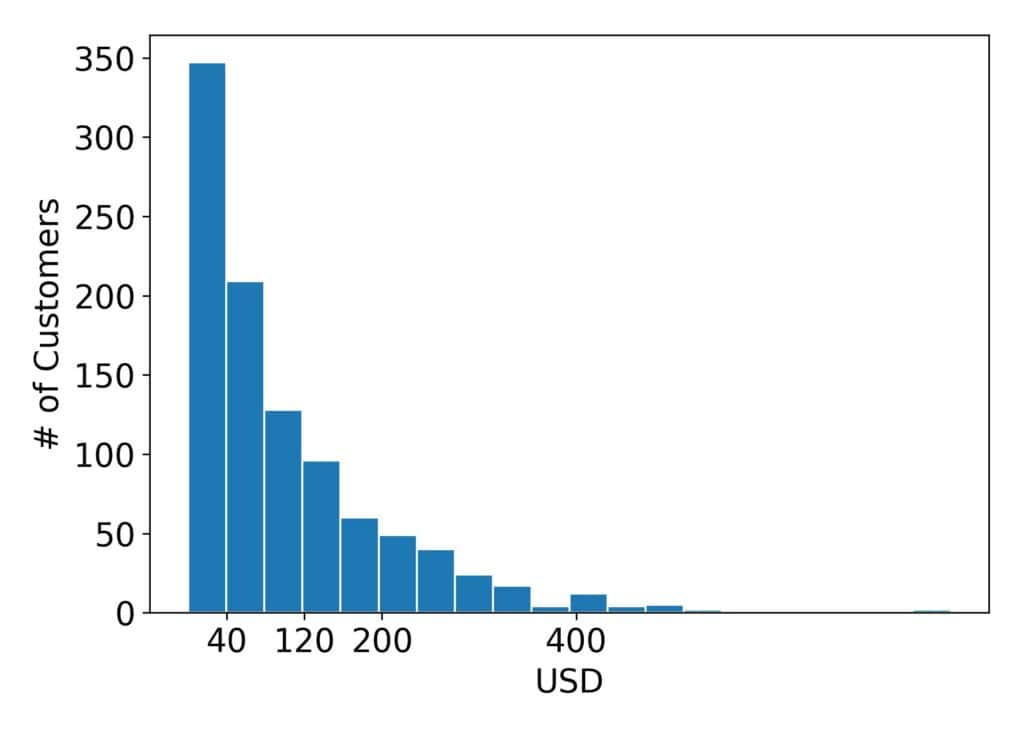
As we see, many customers spend USD 40 or less, but very few spend over USD 1000.
2.1. Math
An exponential distribution has a parameter  . It quantifies the speed at which the occurrence probabilities of values decrease. The distribution’s probability density function (PDF) is:
(1) 
and its cumulative density function (CDF) is:
(2) 
The formulae show that the decrease speed (also known as decay) is exponential, hence the name.
3. The Inversion Method
The inversion method uses a property of CDFs: regarded as random variables, they follow the uniform distribution over ![[0, 1]](/wp-content/ql-cache/quicklatex.com-944fdd98d4f1854c8720f98d8b20b6ad_l3.svg "Rendered by QuickLaTeX.com") :
: ![\mathrm{U}[0, 1]](/wp-content/ql-cache/quicklatex.com-f33ea001571d46797c4efd3a8e56e23d_l3.svg "Rendered by QuickLaTeX.com") . What does that mean? Well, if we sample a lot of numbers
. What does that mean? Well, if we sample a lot of numbers  from an exponential distribution and draw a histogram of the corresponding CDFs, we’ll see a uniform PDF.
But, the converse is also true. If we sample  uniform values
  from
from ![\boldsymbol{\mathrm{U}[0, 1]}](/wp-content/ql-cache/quicklatex.com-c0906017ae084cee07fa9e2dc5c36983_l3.svg "Rendered by QuickLaTeX.com") and calculate the inverses
and calculate the inverses  , we’ll get numbers from the exponential distribution with the decay parameter
  ,
, ![\mathrm{Exp}[\lambda]](/wp-content/ql-cache/quicklatex.com-1083c2e50c4f13a47b09921bd3411f9f_l3.svg "Rendered by QuickLaTeX.com") .
.
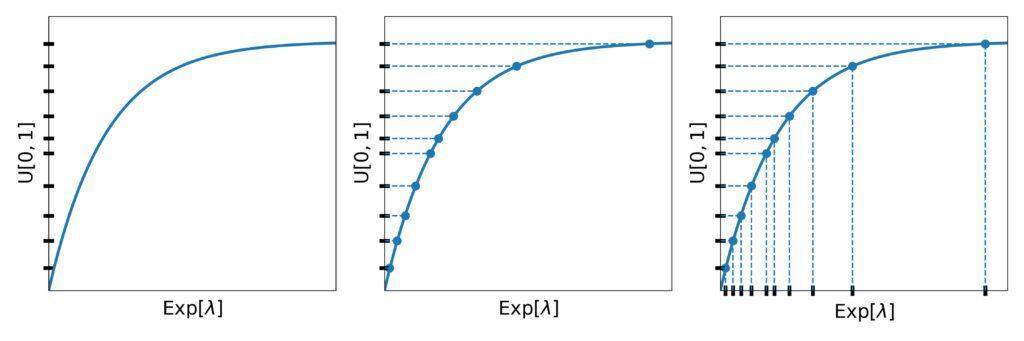
This method has a straightforward geometric interpretation. As the first step, we place the  values on the
  -axis. Then, we find the points of the
  line whose -values are equal to the drawn . The found points’
  -values are the exponential numbers we wanted to draw:
To use the method in programs, we need the inverse  of the exponential CDF. We can derive it analytically:
(3) 
3.1. Pseudocode
Here’s the pseudocode of the inversion method:
algorithm InversionMethod(λ, n):
    // INPUT
    //    λ = the decay parameter of the target exponential distribution
    //    n = how many numbers to draw from it
    // OUTPUT
    //    sample = an array of n numbers from the exponential distribution with the decay λ

    sample <- initialize an empty array

    for i <- 1 to n:
        u <- draw a random number from U[0, 1]
        x <- - (1 / λ) * ln(1 - u)
        append x to sample

    return sample
All we need is numbers from , and the inversion method can transform them to follow ![\boldsymbol{\mathrm{Exp}[\lambda]}](/wp-content/ql-cache/quicklatex.com-3154c5a1bacf18c22580dcc1daa225d7_l3.svg "Rendered by QuickLaTeX.com") for any
for any  .
.
Since  comes from , the difference
  also follows . So, some implementations skip the subtraction step:
(4) 
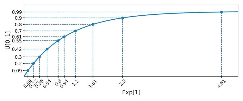
3.2. Example
Let’s say we want ten numbers from ![\mathrm{Exp}[1]](/wp-content/ql-cache/quicklatex.com-84ad07285eb64bf7d5c8605a86c3ae6f_l3.svg "Rendered by QuickLaTeX.com") .
.
First, we draw ten values from ![U[0, 1]](/wp-content/ql-cache/quicklatex.com-d212cb6090d509fb1d4fa0ed2c229fb4_l3.svg "Rendered by QuickLaTeX.com") . For instance, let them be
. For instance, let them be  .
.
Then, we calculate the inverses:

That way, we get ten numbers from :
4. Rejection Sampling
To use the inversion method, we need the inverse  . However, many distributions don’t have an invertible CDF, e.g., the normal distributions. Further, even if we can derive the inverse analytically, it may be too complex to compute efficiently, or we may not have an implementation in our software.
In such cases, we can apply rejection sampling. It uses the PDF plot of the target distribution and selects points from it randomly. If a selected point is below the PDF line, the method keeps its -coordinate. Otherwise, it rejects it. We repeat this step until collecting the desired number of samples.
Here’s the visual representation of rejection sampling for :
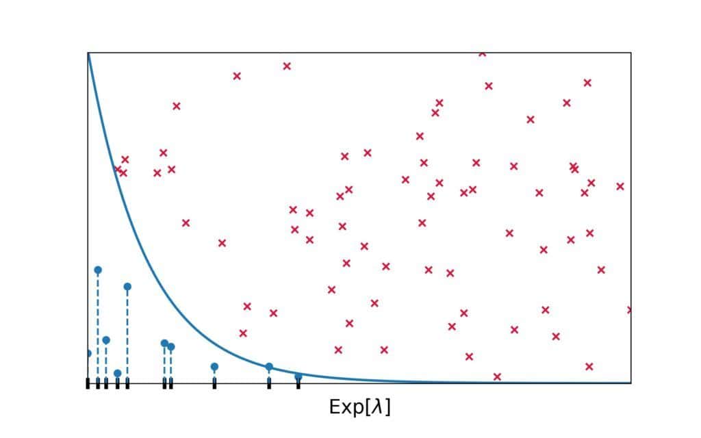
Red crosses represent the rejected points, whereas blue circles denote those we kept. As we see, there are more accepted -values under the regions with higher overall densities.
Why does rejection sampling work? Since the PDF has high values in the high-density regions, they have a greater chance of capturing a randomly drawn point.
4.1. Pseudocode
Here’s the pseudocode of rejection sampling adapted to the exponential distribution :
algorithm RejectionSampling(λ, n, r):
    // INPUT
    //    λ = the decay parameter of the target exponential distribution
    //    n = how many numbers to draw from it
    //    r = the upper bound for x-coordinates
    // OUTPUT
    //    sample = an array of n numbers from the exponential distribution with the decay λ

    sample <- an empty array
    m <- 0

    while m < n:
        x <- draw a random number from [0, r]
        y <- draw a random number from [0, λ]

        if y <= f_λ(x):
            append x to sample

    return sample
To select a random point in the plot according to a 2D uniform distribution, we can draw the and coordinates independently.
Since the support of ![\mathrm{Exp}[\cdot]](/wp-content/ql-cache/quicklatex.com-105eb3df493bf749d4656c69b867afc3_l3.svg "Rendered by QuickLaTeX.com") is
is ![[0, \infty]](/wp-content/ql-cache/quicklatex.com-2e51c95f5a9e59ca6242306fadc3499b_l3.svg "Rendered by QuickLaTeX.com") , we can propose any non-negative value as . However, using the maximal positive number as the bound would result in many rejected values and poor performance. So, we restrict sampling of the
, we can propose any non-negative value as . However, using the maximal positive number as the bound would result in many rejected values and poor performance. So, we restrict sampling of the  -coordinates to
 ![\boldsymbol{[0, r]}](/wp-content/ql-cache/quicklatex.com-8020811bfa17e4fea98fefdf3854722c_l3.svg "Rendered by QuickLaTeX.com") , where
, where  is a suitable upper bound.
How do we choose ? We can set it to a value that very rarely occurs. For instance,  of is to the left of
  . For
. For  , that is approximately 9.21.
Similarly, we sample  from
from ![\boldsymbol{\mathrm{U}[0, \max{f_{\lambda}}]}](/wp-content/ql-cache/quicklatex.com-8659e46a016ffc3b36bc29927e1a3c83_l3.svg "Rendered by QuickLaTeX.com") . That way, we speed up sampling because we won’t get points that are certainly above the PDF of and have a zero chance of being kept.
. That way, we speed up sampling because we won’t get points that are certainly above the PDF of and have a zero chance of being kept.
Since the maximum density of ![Exp[\lambda]](/wp-content/ql-cache/quicklatex.com-d8512fa81f0195cfbe6894279657a4e9_l3.svg "Rendered by QuickLaTeX.com") is at
is at  and is equal to , we sample -coordinates from
 ![\mathrm{U}[0, \lambda]](/wp-content/ql-cache/quicklatex.com-482329c3bcf8273c0f28130a307ed878_l3.svg "Rendered by QuickLaTeX.com") .
.
4.2. Example
The first several iterations of rejection sampling for generating numbers from could go like this:
 |
|
|
 |
 |
|---|---|---|---|---|
| 1 | 1.17 | 0.73 | 0.31 | reject |
| 2 | 4.38 | 0.11 | 0.01 | reject |
| 3 | 2.61 | 0.47 | 0.07 | reject |
| 4 | 1.72 | 0.98 | 0.18 | reject |
| 5 | 8.68 | 0.64 | 0.0 | reject |
| 6 | 4.79 | 0.01 | 0.01 | keep |
| 7 | 0.65 | 0.67 | 0.52 | reject |
| 8 | 0.38 | 0.43 | 0.68 | keep |
| 9 | 2.68 | 0.92 | 0.07 | reject |
 |
||||
Here, we can see a potential problem rejection sampling can face. It can generate many more points than we need. That can happen if the algorithm draws points mostly above the PDF line.
4.3. Optimization
One way to address this issue is to set to a smaller value. For instance, we can use the  -quantile or
  -quantile of the target . However, trimming the distribution too much skews the generated numbers to the left. If that happened, we wouldn’t sample from , but from a similar yet different distribution.
We can also play with drawing points from the plot. Here, we used a 2D uniform distribution over ![[0, r] \times [0, \lambda]](/wp-content/ql-cache/quicklatex.com-4eceb0b13a9fd6257ed5a810fb62279c_l3.svg "Rendered by QuickLaTeX.com") to sample them, but any distribution would have worked. The only question is how to choose the one that best suits our target distribution.
to sample them, but any distribution would have worked. The only question is how to choose the one that best suits our target distribution.
5. Conclusion
In this article, we talked about sampling from an exponential distribution. We presented two techniques: the inversion method and rejection sampling.
The inversion method uses the inverse of the exponential CDF. Rejection sampling doesn’t require the inverse but can take longer.