Yes, we're now running our only Summer Sale. All Courses are 30% off until 20th July, 2026:
Which Sorting Algorithm to Use?
Last updated: May 23, 2025

Learn through the super-clean Baeldung Pro experience:
>> Membership and Baeldung Pro.
No ads, dark-mode and 6 months free of IntelliJ Idea Ultimate to start with.
1. Overview
In this tutorial, we’ll discuss various sorting algorithms and the purpose of using them in a particular circumstance. Though sorting algorithms have a general aim of sorting, each has its own disadvantages and advantages. Some algorithms overcame the issues that prevailed in the existing ones.
The problems are based on the additional space required, time complexity, and the ability to handle complex or huge data. An algorithm is applied in each case based on how it deals with a data structure such as arrays, linked lists, stack, or queues. Typical applications are e-commerce, database management systems, or graph traversal.
2. Sorting Algorithms
Sorting is the process of arranging the elements in order (usually ascending). Applications that have to search a particular element require organized data. In this section, we’ll see the various sorting algorithms and their complexities.
2.1. Merge Sort
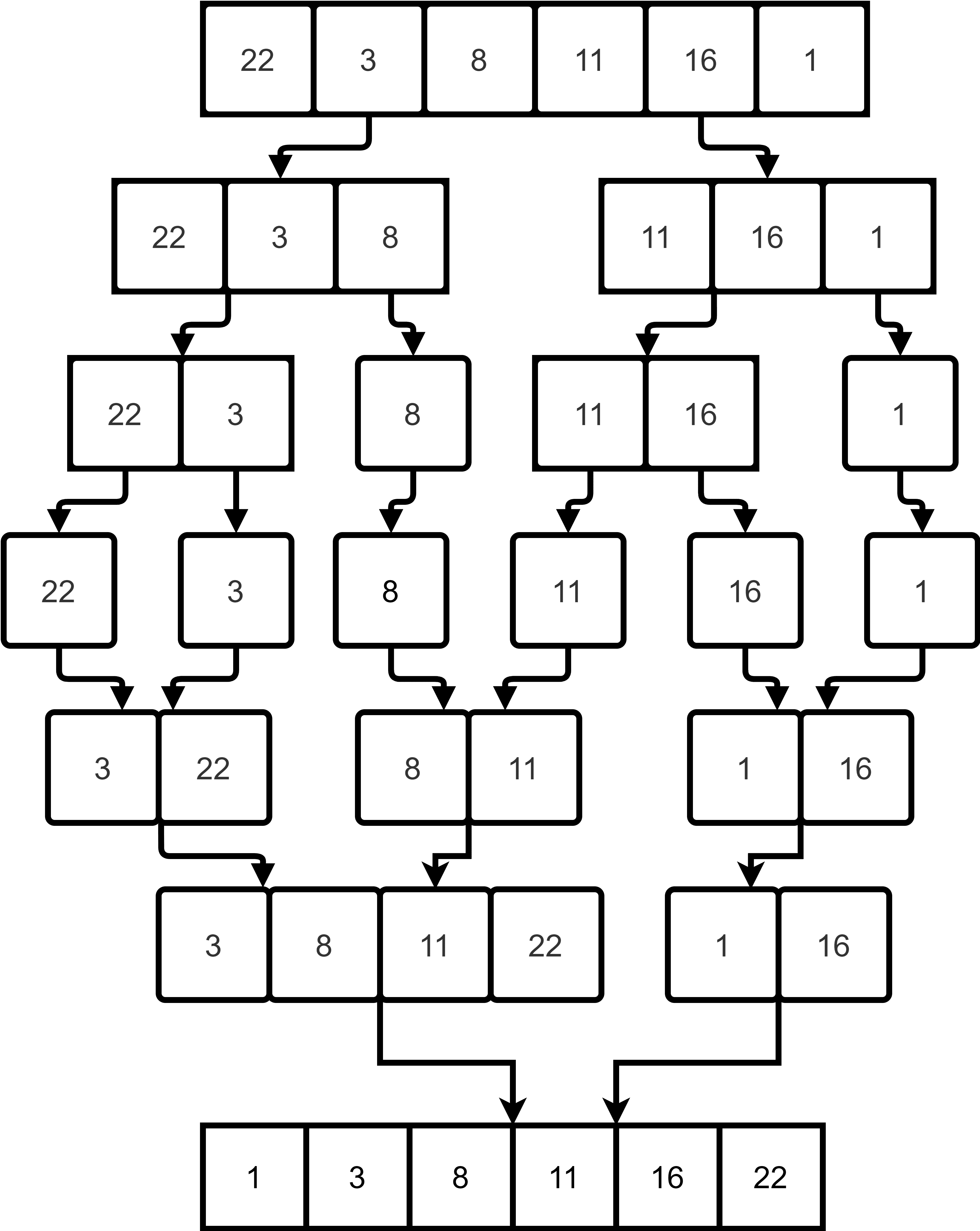
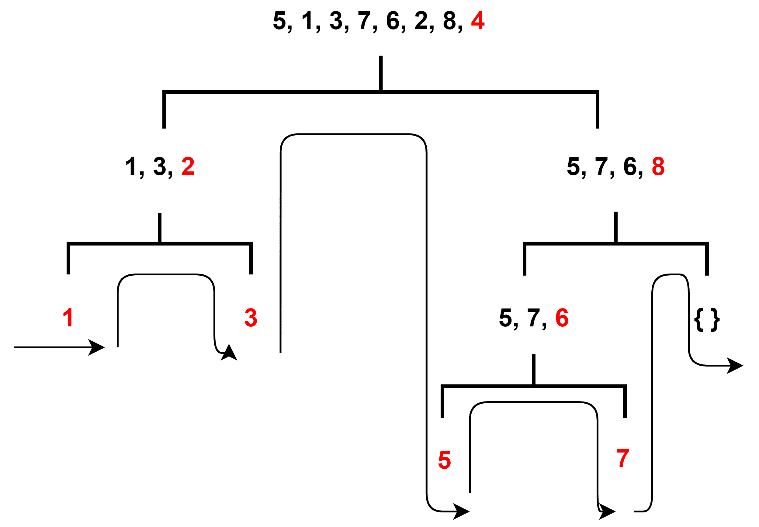
Merge sort, invented by John Von Neumann, follows the divide and conquer method to sort the  number of elements. Firstly, the values go through iterative splitting into equal-sized groups (each group at that iteration containing
  elements) until each group has a single value. Then the elements merge in a reverse manner to the splitting process. Merging gradually sorts the data in that merged group for every iteration. Finally, producing a set of sorted elements:
Merge sort is suitable for data structures that are accessed in series. Tape drives are the best example where the CPU has access to the data in sequential order. It is also used in the field of e-commerce to keep track of user interests using inversion.
Merge sort performs the same complete process regardless of the data. Its best, average, and worst-case for time complexity is  where is the number of elements sorted. The space complexity is
  for additional space and
  when implemented using linked lists.
The data is copied to a separate list at each iteration. Therefore, it is not preferred for arrays, especially with big datasets. Linked lists are better since insertion does not require extra space.
2.2. Bubble Sort
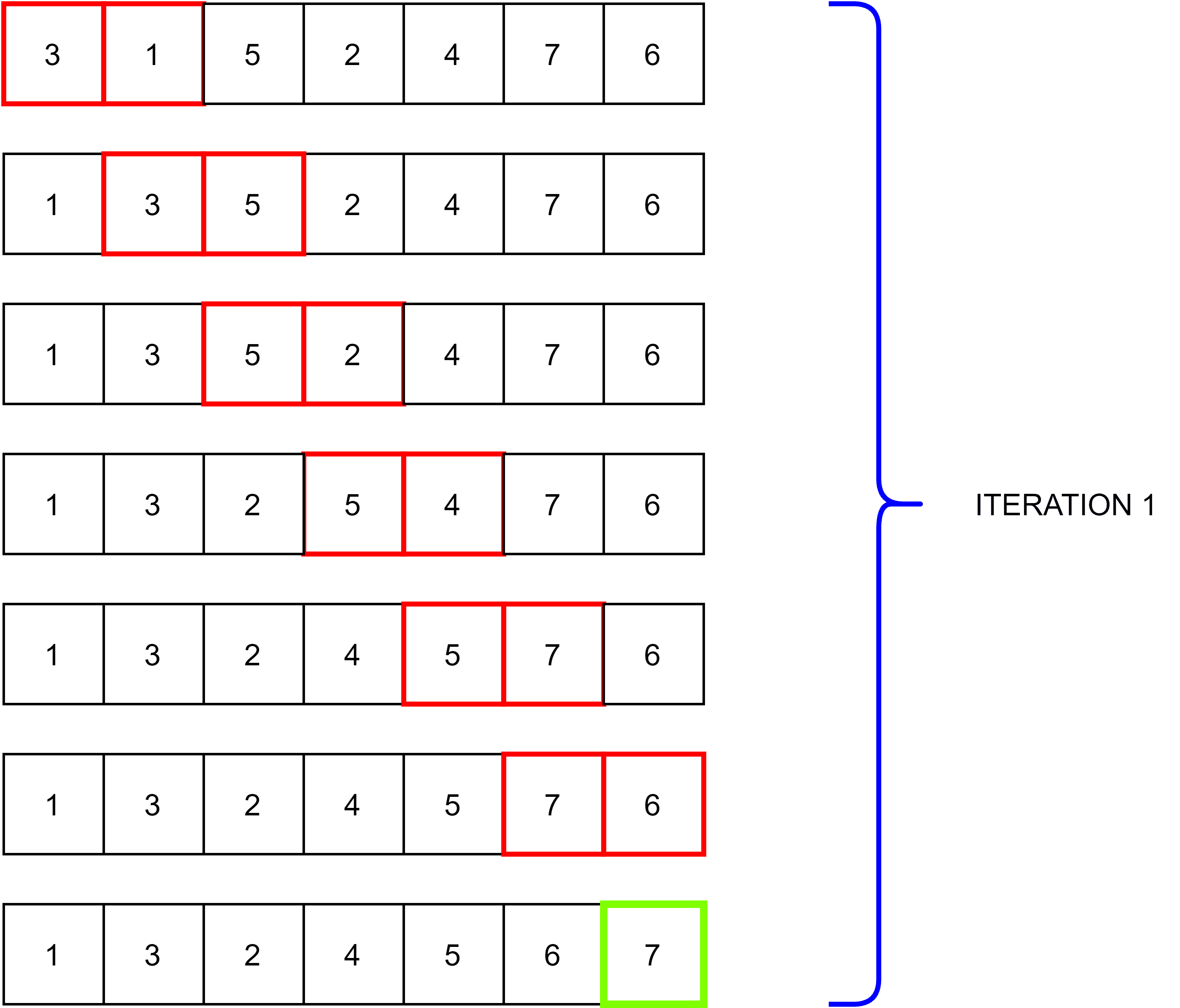
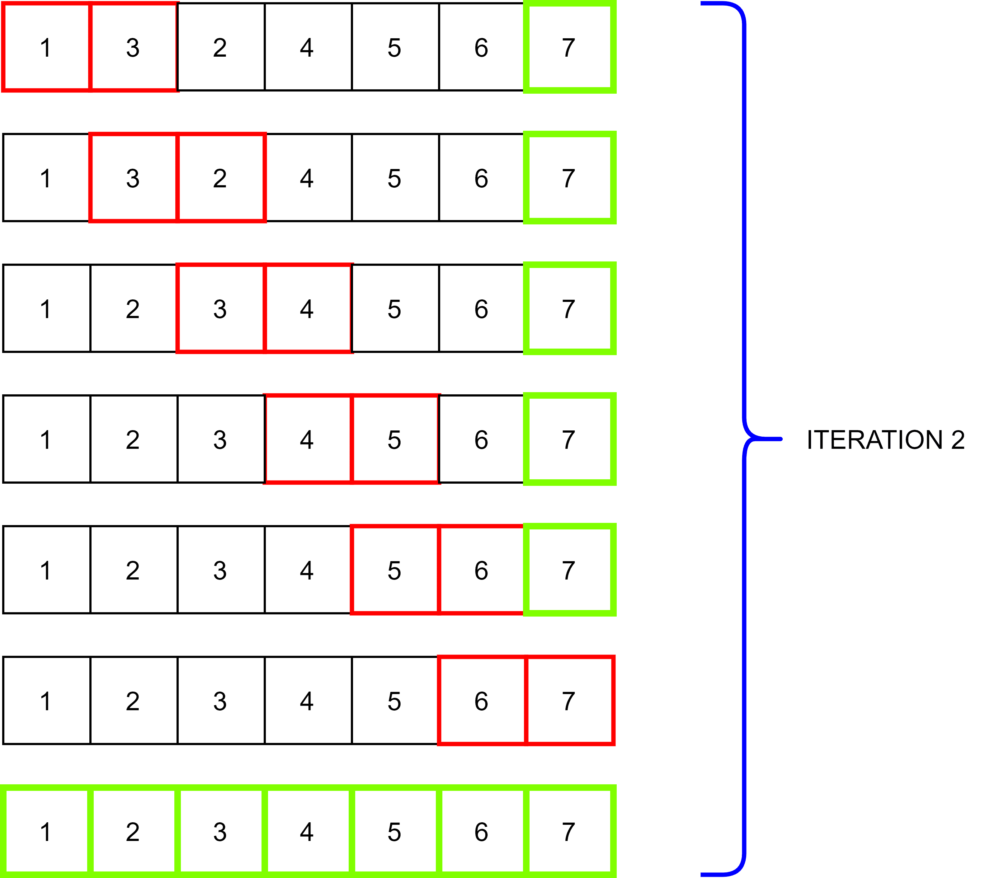
Bubble sort is one of the simplest sorting algorithms which came into usage by Iverson. It sorts by comparing each pair of adjacent elements and swapping them if they are not in ascending order. The process takes place for various iterations to sort completely. As the iterations proceeds, the list starts falling in order from the last element:
Smaller lists sort using bubble sort due to its simplicity, where it just takes  to complete the sorting. In computer graphics, it is used for the polygon filling algorithm to arrange the coordinates of lines in order.
For a sorted list, the best case for time complexity is . The average and worst-case is  , where the worst-case situation is the elements in descending order. In the worst-case scenario, the maximum number of pairs swap to reach the end at every iteration. Bubble sort is still used for a basic understanding of the sorting algorithms and smaller element sets.
2.3. Selection Sort
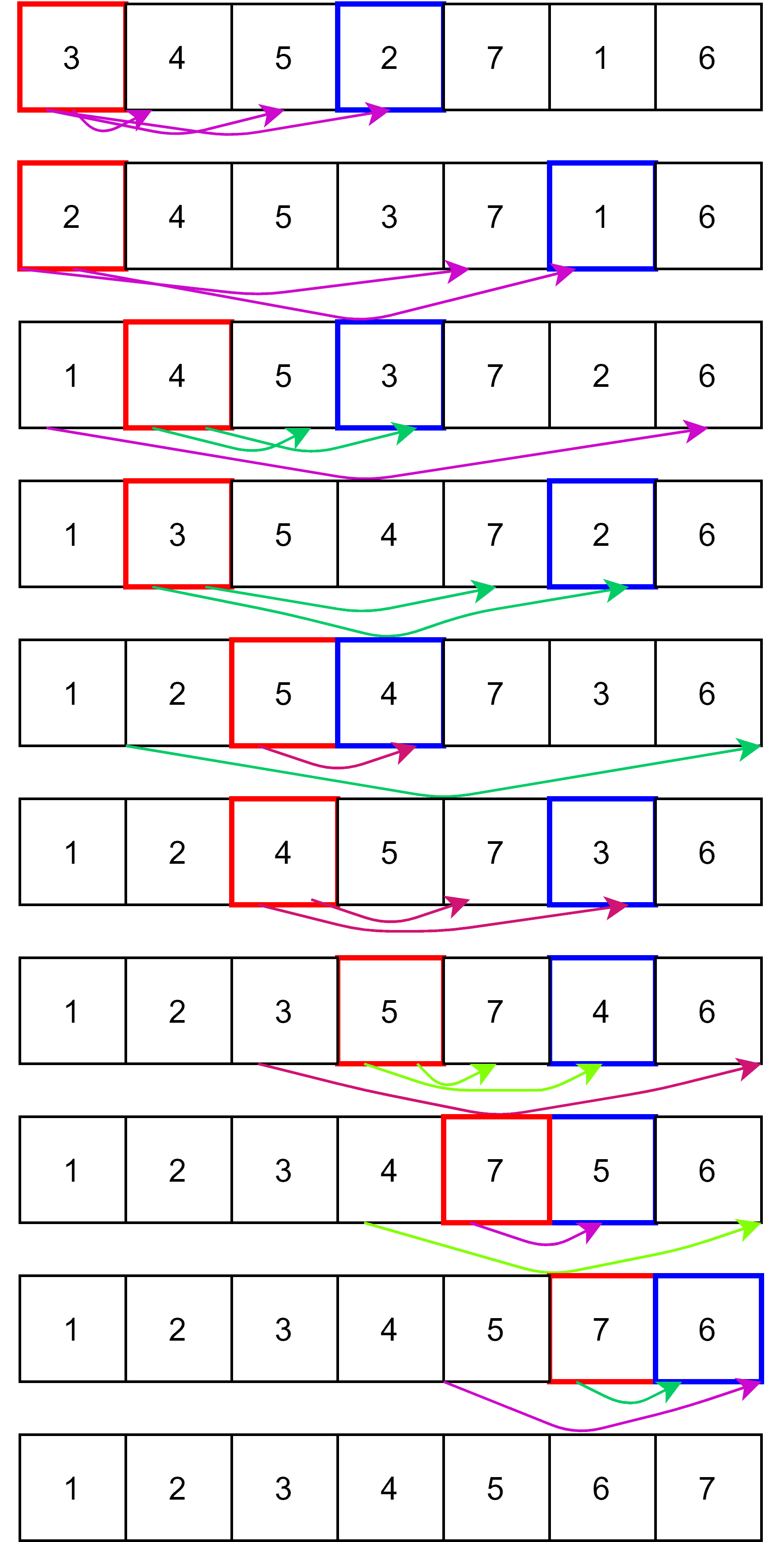
Selection sort is a sorting procedure that proceeds by finding the minimum element and replacing the values. The algorithm starts by comparison from the item at the first location. It is checked with the others to see if a smaller value is present in any other position. If yes, it swaps the elements, making sure to place the smallest number in the first location.
For example, element  at the first location is checked against each element to its right. If is less than any other element
  , then remains at that location. Otherwise, swaps with , and now is compared with the rest of the elements. This procedure finally gives the sorted order of the elements:
The algorithm compares every element for every location, so the time complexity of the selection sort is . On the other hand, the space complexity is . It sorts faster in a small set of items. Just like the bubble sort, it’s useful for learning the concept of sorting.
2.4. Quicksort
Quicksort is another sorting method using the divide and conquer technique, developed by Tony Hoare. The algorithm repeatedly splits the elements based on a pivot number chosen (the same position throughout the sorting process). It continually does this to the subgroups until it reaches a group with a single element. The method splits the groups into two subgroups, according to whether they are less or greater than the pivot number:
Best and average-case time complexity are . The best case is choosing a pivot number that is the median value every time.
The worst case is when the pivot number selected is the smallest or greatest number every time. This state might happen when the elements are sorted in ascending or descending order. The worst-case time complexity is .
The space complexity of this sorting method is  . Even though quicksort doesn’t require much extra space, it isn’t that advisable for a larger dataset.
Quicksort works faster in a virtual environment, where the memory space that’s not part of primary memory yet seems like one while running a process. It suits well for arrays where it’s easier to access elements based on location and doesn’t require extra storage.
2.5. Heapsort
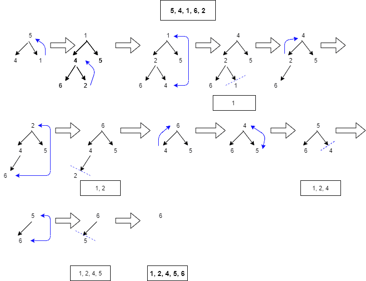
J.W.J. Williams developed the method heapsort, which sorts elements by constructing a binary tree structure. There are two types of tree forms: max-heap tree and min-heap tree. When the parent node is greater than the children node, it is called a max heap tree. When the parent node is less than the children node, then it’s called a min-heap tree.
Heapsort proceeds by three main actions: heapify, swap, and insert.
- During heapify, the tree is checked after every insertion of a new node whether the tree satisfies max-heap or min-heap tree structure.
- After the tree is in heap form, the first element swaps with the last bit
- Finally, it inserts the end element in the updated tree into the sorted output list
These three steps repeatedly continue until the root node is left, inserted into the output list to obtain the sorted elements:
Systems that require security and embedded systems use heapsort. Since it generally does the same procedure to sort the elements, its time complexity at all cases is .
Since the space complexity is , it is well recommended for sorting linked lists. The complexity of heapsort increases logarithmically when elements increase, which makes it suitable for huge datasets.
2.6. Insertion Sort
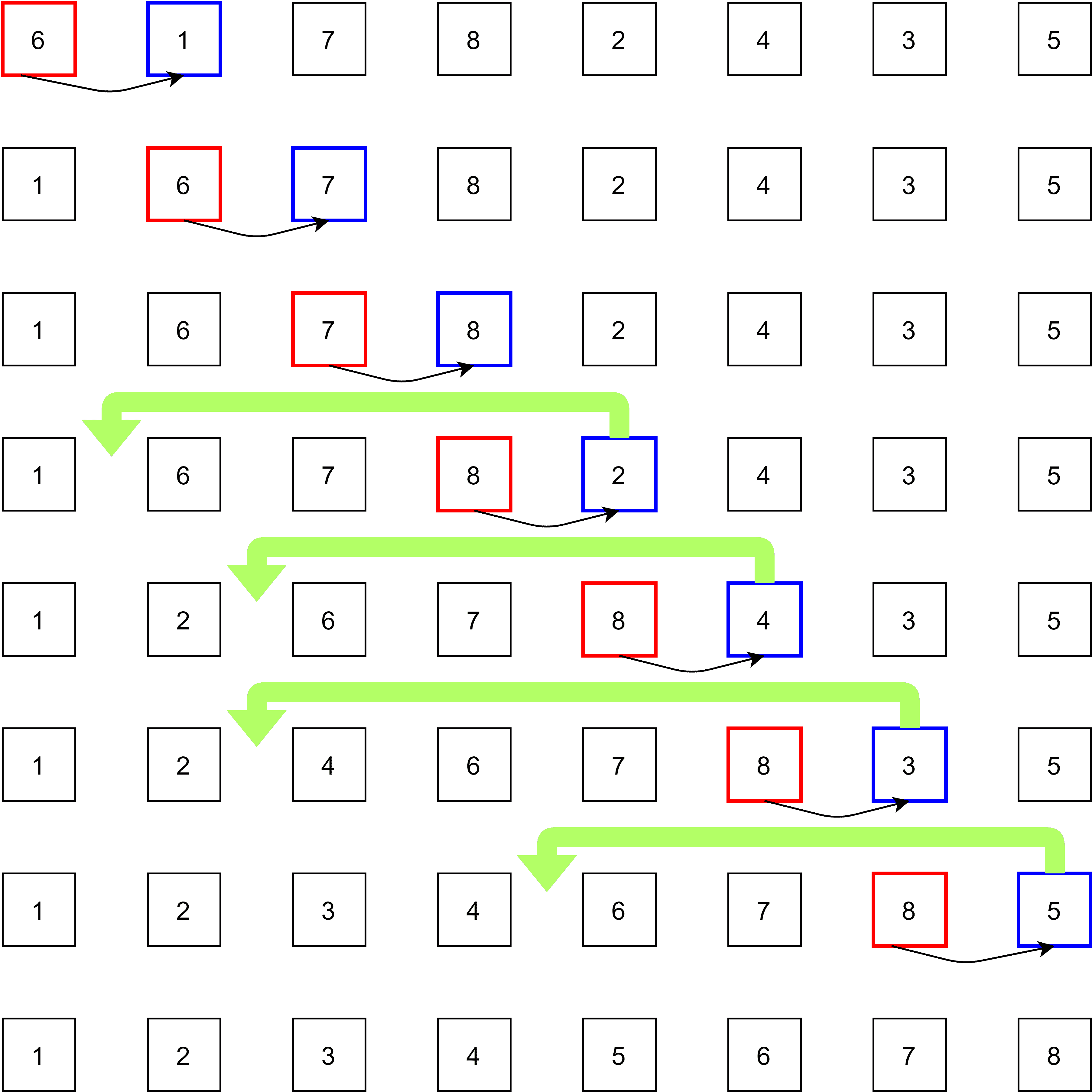
The insertion sort is a simple iterative sorting method introduced by John Mauchly. Insertion sort follows three steps: Compare, Move, and Place.
The insertion sort compares one item with its successor in every iteration and steps are:
- The element
![array[a]](/wp-content/ql-cache/quicklatex.com-7c9d94cfb87409d9cbbcd204e02da4f5_l3.svg "Rendered by QuickLaTeX.com") compares whether its successor
compares whether its successor ![array[a+1]](/wp-content/ql-cache/quicklatex.com-4eb9b40a81e4b69a1cd67dedd175db48_l3.svg "Rendered by QuickLaTeX.com") is greater than it
is greater than it - If yes, it is left as it is and now the successor element is checked with its adjacent element
![array[a+2]](/wp-content/ql-cache/quicklatex.com-d1fb703d3d27e31940e00ea50e892520_l3.svg "Rendered by QuickLaTeX.com")
- Otherwise, the element moves one position up and gives space for insertion
- While the successive element is compared to the elements before it and placed at the correct position in the list
- While placing, an item
 is placed in such a position where its predecessors are lesser than
The worst and average case for time complexity is , where every element moves to build a sorted list and the rest of the bits shift every time. The best-case scenario is when it’s a sorted list and the time complexity is . And the space complexity for insertion sort is . Insertion sort can be used for smaller datasets and almost sorted lists in a larger dataset.
2.7. Introsort
Introsort invented by David Musser is a hybrid sorting algorithm that does not have any separate sorting technique, yet remarkable due to its sorting strategy. The main feature of intro sort is choosing between insertion sort, quicksort, and heapsort based on the dataset.
Each sorting algorithm has its advantages and disadvantages. Introsort uses a suitable sorting algorithm depending upon the data set. Since insertion sort is good with more minor data, it sorts that kind of data. Quicksort is good when the pivot element is an intermediate value obtained by finding the median. And heapsort is used when the iterations get higher. Still, introsort has the main disadvantage that it cannot put data into the array.
3. Summary
Here is a table summarizing when each sorting algorithm is preferred.
| Which algorithm to use | ||
|---|---|---|
| Algorithm Name | Description | When to use |
| Merge Sort | First, the values split until single-element groups and sorts sub-group while gradually merging | Used for sorting linked list |
| Bubble Sort | Compares adjacent element pairs and swaps if they are not ascending | Good for understanding sorting and sort small data set |
| Selection Sort | For each location, it checks whether it’s less than the elements to its right | Beneficial to learn sorting algorithms |
| Quick Sort | Repeatedly splits elements based on chosen pivot number | Used for sorting arrays and medium-sized data set |
| Heap Sort | Proceeds by heapify, swap and insert | Ideal for big data sets |
| Insertion Sort | Sorts by comparing, moving, and placing | Used to sort small data set and check already sorted list |
| Intro Sort | Chooses between other sorting algorithm based on data set | Uses insertion sort to sort small dataset, quicksort when the pivot is the median, and heap sort for sorting large dataset |
4. Conclusion
In this tutorial, we have defined various sorting algorithms and explained their sorting procedures. Their time and space complexities have been provided and thereby giving the merits and demerits of each algorithm. As a result of this, the readers will finally obtain the application areas of those sorting algorithms.