

Learn through the super-clean Baeldung Pro experience:
>> Membership and Baeldung Pro.
No ads, dark-mode and 6 months free of IntelliJ Idea Ultimate to start with.
Learn through the super-clean Baeldung Pro experience:
>> Membership and Baeldung Pro.
No ads, dark-mode and 6 months free of IntelliJ Idea Ultimate to start with.
In this tutorial, we’ll learn what a priority queue is and understand how it works. Priority queues have many applications on other algorithms such as Dijkstra and scheduling algorithms. Priority queues are very important to systems that juggle multiple programs and their execution (programs are chosen to run based on their priority). They are also very important to networking systems, like the internet, because they can help prioritize important data to make sure it gets through faster.
A priority queue is a special type of queue. Each queue’s item has an additional piece of information, namely priority. Unlike a regular queue, the values in the priority queue are removed based on priority instead of the first-in-first-out (FIFO) rule. The following example illustrates a priority queue with an ordering imposed on the values from least to the greatest: 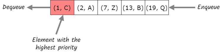 Here,
Here,  , etc. denotes the value of items while
  , etc. denotes the priority of items. So the item with the highest priority in this example is
  (with the priority of 1) that is removed first. And the lowest priority item,
  (with the priority of 19), will be removed at the end of the process. In this tutorial, from now on, we’ll use priority as the value of items since other information can be easily attached to the queue’s elements. The main operations on a priority queue include:
A priority queue is an extension of a queue that contains the following characteristics:
There are two types of priority queues:
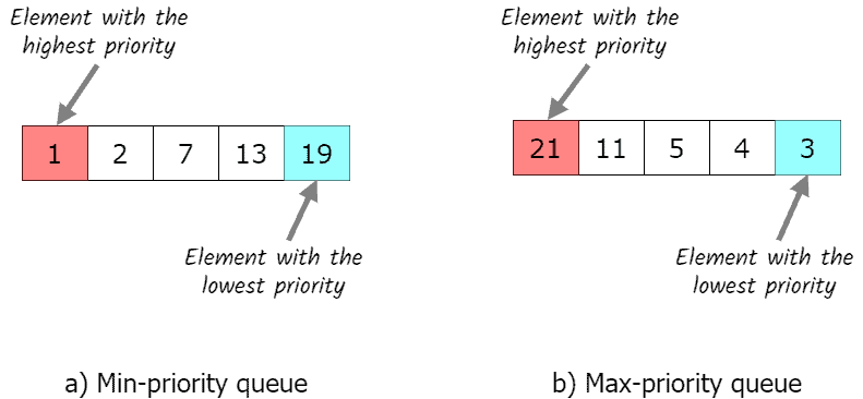 In both types, the priority queue stores a collection of elements and is always able to provide the most “extreme” element, which is the only way to extract the value from the priority queue. For the remainder of this tutorial, we’ll discuss max-priority queues. Min-priority queues are analogous.
There are different ways to implement a priority queue. The main ways include array, linked list, binary search tree (BST), and binary heap tree. The heap data structure is the most efficient way to implement a priority queue. Before diving deeper into the heap data structure, let’s briefly discuss the efficiency of each implementation approach on basic operations of queues:
| Unordered Array | Sorted Array | Unordered Linked List | Sorted Linked List | BST | Heap | |
|---|---|---|---|---|---|---|
| add |  |  | | |  |  |
| peek | | | | | | |
| remove | | | | | | |
A binary heap is a type of binary tree (but not a binary search tree) that has the following properties:
Throughout this tutorial, we’ll be using examples of a max heap. Let’s examine the following example to understand the heap structure better: 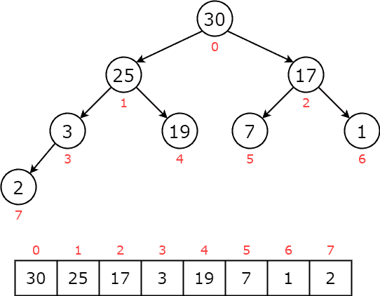 For each node
  , the left child will be at
  , and the right child will be at
  . The parent will be at
  (except for the root node at
  ). For a more in-depth overview of the heap data structure, we can read the article which explains Heap Sort in Java.
The common operations that we can perform on a priority queue include insertion, deletion, and peek. We’ll use a binary heap to maintain a max-priority queue. The item at the root of the heap has the highest priority among all elements. If we want to add a new node to a binary heap, we need to ensure that our two properties of the heap are maintained after the new node is added. At first, we insert the new item at the end of the priority queue. If it is found greater than its parent node, elements are swapped. This process continues until the new item is placed in the correct position. Let’s go through an example to understand the insertion process. If we add  to the priority queue, we end up with:
 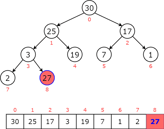 We notice that is greater than its parent
  , so we swap them:
 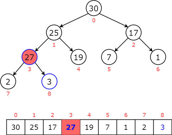 Then, is still greater than its new parent
  , so we swap them:
 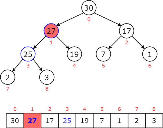 Now, we notice that is smaller than its parent, so we stop and reach our priority queue:
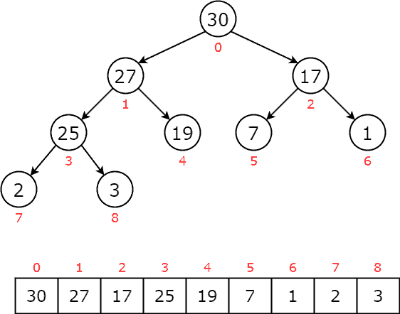
The following code shows the details of the insertion function:
algorithm insertIntoPriorityQueue(heap, n, val):
    // INPUT
    //    heap = the priority queue
    //    n = the size of the priority queue
    //    val = the priority value of the new item
    // OUTPUT
    //    Returns the priority queue after inserting the new item and re-heapifying

    i <- n
    heap[n] <- val
    n <- n + 1
    // Heapify the tree
    while i > 0 and heap[(i - 1) / 2] < heap[i]:
        swap(heap[(i - 1) / 2], heap[i])
        i <- (i - 1) / 2
    return heap
Next, we can remove the maximum element from the priority queue. As we know, the root node is the item with the highest priority in a max heap. When removing the root node, we replace it with the last item of the priority queue. Then, this item is compared with the child nodes and swap with the greater one. It keeps moving down the tree until the heap property is restored. Now, let’s apply to an example to understand how this process works. First, we replace the root node  with the last item :
 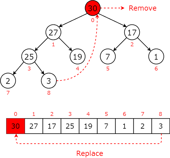 The new priority queue is now violent the max heap’s property where the root node is smaller than its children:
 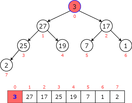 Then, we swap node with the greater child until it reaches the leaf or greater than both children:
 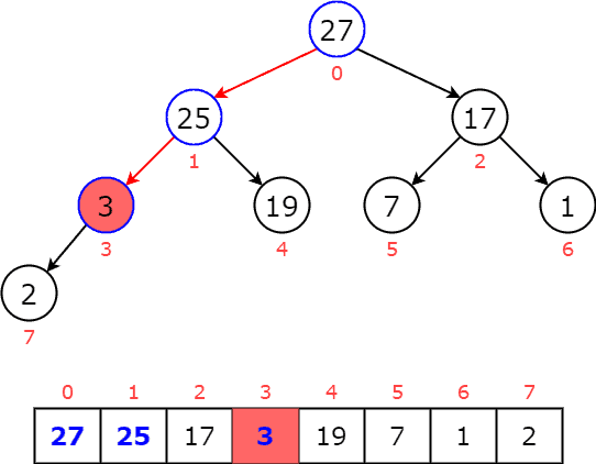 Now, is greater than its child of
  , we stop and reach our priority queue:
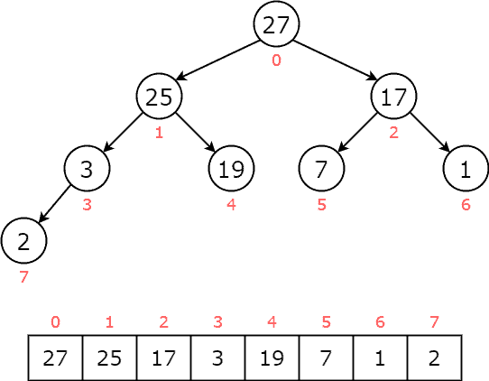
The following code shows the details of the deletion function:
algorithm removeFromPriorityQueue(heap, n):
    // INPUT
    //    heap = the priority queue
    //    n = the size of the priority queue
    // OUTPUT
    //    The item with the highest priority is removed from the queue

    if n = 0:
        // if the priority queue is empty
        return -1

    // save the max priority value to return later
    max <- heap[0]
    heap[0] <- heap[n - 1]
    n <- n - 1
    i <- 0

    // Heapify the tree
    while 2 * i + 1 < n:
        left <- 2 * i + 1
        right <- 2 * i + 2
        if heap[left] > heap[right] or right >= n:
            selected_child <- left
        else:
            selected_child <- right
        if heap[i] >= heap[selected_child]:
            break
        swap(heap[i], heap[selected_child])
        i <- selected_child
    return max
If we want to peek and see the largest node in a heap quickly, that is easy. Just return a pointer to the root:
algorithm peekPriorityQueue(heap, n):
    // INPUT
    //    heap = the priority queue
    //    n = the size of the priority queue
    // OUTPUT
    //    The item with the highest priority without removing it from the queue

    if n = 0:
        // if the priority queue is empty
        return -1

return heap[0]For insertion, we may have to heapify the entire heap data structure. So, while the insertion process only takes O(1) time, the heapify process will take  . The same goes for deletion. We know where the max priority value is, but remaking the heap still takes time. These are guaranteed worst-case efficiency since a binary heap always guarantees a complete tree. The time complexity to extract the value from a priority queue is since we only need to peek at the root node of the heap.
Priority queues are widely applied on other algorithms as well as in real-world systems. The main applications include:
In this article, we discussed the data structure called a priority queue. We’ve learned the definition and characteristics of a priority queue. We’ve learned how to implement a priority queue using a heap data structure. Finally, we discussed the complexity of the priority queue’s operation and the application of priority queues.